Proxy dataset - MTG Sentinel-4 UV-Visible-Near infrared (UVN) spectrometer - Nitrogen Dioxide (NO2)
Contents
Proxy dataset - MTG Sentinel-4 UV-Visible-Near infrared (UVN) spectrometer - Nitrogen Dioxide (NO2)
The geostationary Sentinel-4 mission will provide hourly data on tropospheric constituents over Europe for air quality applications. The target species of the Sentinel-4 mission include key air quality parameters such as nitrogen dioxide, ozone, sulphur dioxide, formaldehyde, glyoxal, and aerosols. These species will be monitored by the Sentinel-4 UVN instrument aboard the MTG Sounder satellite.
This notebook provides you an introduction to European Air Quality Forecasts from the Copernicus Atmosphere Monitoring Service (CAMS) and ERA5 reanalysis data from the Copernicus Climate Change Service (C3S). A combination of these two dataset can be used as a proxy for data from the geostationary Sentinel-4 mission.
The event that this notebook hightlights are the fires in southern Italy and in Greece during August 2021.
Nitrogen dioxide is a useful indicator of smoke presence and transport.
Basic Facts
CAMS European Air Quality Forecasts
Spatial resolution: 0.1° x 0.1°
Spatial coverage: Europe
Temporal resolution: 1-hourly up to leadtime hour 120
Temporal coverage: three-year rolling archive
Data format: GRIB or zipped NetCDF
C3S ERA5 reanalysis
Spatial resolution: 0.25° x 0.25°
Spatial coverage: Global
Temporal resolution: 1-hourly
Temporal coverage: since 1950
Data format: GRIB or NetCDF
How to access the data
Copernicus Atmosphere Data Store (ADS)
CAMS European air quality forecasts are available for download via the Copernicus Atmosphere Data Store (ADS). You will need to create an ADS account here.
Data from the ADS can be downloaded in two ways:
manuallyvia the ADS web interfaceprogrammaticallywith a Python package called cdsapi (more information)
Copernicus Climate Change Service
C3S ERA5 reanalysis are available for download via the Copernicus Climate Data Store (CDS). You will need to create a CDS account here.
Data from the CDS can be downloaded in two ways:
manuallyvia the CDS web interfaceprogrammaticallywith a Python package called cdsapi (more information)
Load required libraries
import os
import xarray as xr
import numpy as np
import netCDF4 as nc
import pandas as pd

# Python libraries for visualization
%matplotlib inline
import matplotlib.pyplot as plt
import matplotlib.colors
from matplotlib.cm import get_cmap
from matplotlib import animation
from matplotlib.axes import Axes
import cartopy.crs as ccrs
from cartopy.mpl.gridliner import LONGITUDE_FORMATTER, LATITUDE_FORMATTER
import cartopy.feature as cfeature
from cartopy.mpl.geoaxes import GeoAxes
GeoAxes._pcolormesh_patched = Axes.pcolormesh
from IPython.display import HTML

import warnings
warnings.simplefilter(action = "ignore", category = RuntimeWarning)
warnings.simplefilter(action = "ignore", category = UserWarning)
Load helper functions
%run ../functions.ipynb
CAMS European air quality forecasts
Retrieve CAMS European air quality forecasts from the Atmosphere Data Store
[OPTIONAL] The first step is to programmatically download the Nitrogen Dioxide analysis information as part of the European Air Quality Forecasts dataset. This step is optional because we have already downloaded the data for you, which is why the following code is commented out. The retrieve request below requests the following data:
Date: 7 August 2021
Variable: Nitrogen Dioxide
Model: EURAD-IM
Type: Analysis
Pressure level: [5000, 3000, 2000, 1000, 500, 250, 50, 0]
Spatial resolution: 0.1 deg x 0.1 deg
Temporal resolution: hourly
Format: netcdf
The data is downloaded with the filename 20210807_euradim_no2.nc.
Note: Replace the hashes with your ADS credentials. You can find them here, once you are logged in.
# URL = '###########################'
# KEY = '############################'
'''
import cdsapi
c = cdsapi.Client(url=URL, key=KEY)

c.retrieve(
    'cams-europe-air-quality-forecasts',
    {
        'model': 'euradim',
        'date': '2021-08-07/2021-08-07',
        'format': 'netcdf',
        'type': 'analysis',
        'variable': 'nitrogen_dioxide',
        'level': [
            '0', '1000', '2000',
            '250', '3000', '50',
            '500', '5000',
        ],
        'leadtime_hour': '0',
        'time': [
            '00:00', '01:00', '02:00',
            '03:00', '04:00', '05:00',
            '06:00', '07:00', '08:00',
            '09:00', '10:00', '11:00',
            '12:00', '13:00', '14:00',
            '15:00', '16:00', '17:00',
            '18:00', '19:00', '20:00',
            '21:00', '22:00', '23:00',
        ],
    },
    './20210807_euradim_no2.nc')
'''
"\nimport cdsapi\nc = cdsapi.Client(url=URL, key=KEY)\n\nc.retrieve(\n 'cams-europe-air-quality-forecasts',\n {\n 'model': 'euradim',\n 'date': '2021-08-07/2021-08-07',\n 'format': 'netcdf',\n 'type': 'analysis',\n 'variable': 'nitrogen_dioxide',\n 'level': [\n '0', '1000', '2000',\n '250', '3000', '50',\n '500', '5000',\n ],\n 'leadtime_hour': '0',\n 'time': [\n '00:00', '01:00', '02:00',\n '03:00', '04:00', '05:00',\n '06:00', '07:00', '08:00',\n '09:00', '10:00', '11:00',\n '12:00', '13:00', '14:00',\n '15:00', '16:00', '17:00',\n '18:00', '19:00', '20:00',\n '21:00', '22:00', '23:00',\n ],\n },\n './20210807_euradim_no2.nc')\n"
Load and browse CAMS European air quality forecasts
The next step is to open the NetCDF file as xarray Dataset. You can use the function open_dataset() to open a single NetCDF file. The dataset has four dimensions (longitude, latitude, level and time). A closer look at the coordinates shows that the longitude coordinates are on a grid from [0, 360]. In a next step, we can bring the longitude values to a [-180, 180] grid.
file_cams = xr.open_dataset('../data/cams/2021/20210807_euradim_no2.nc')
file_cams
<xarray.Dataset>
Dimensions:    (longitude: 700, latitude: 420, level: 8, time: 24)
Coordinates:
  * longitude  (longitude) float32 335.0 335.1 335.2 335.4 ... 44.75 44.85 44.95
  * latitude   (latitude) float32 71.95 71.85 71.75 71.65 ... 30.25 30.15 30.05
  * level      (level) float32 0.0 50.0 250.0 500.0 1e+03 2e+03 3e+03 5e+03
  * time       (time) timedelta64[ns] 00:00:00 01:00:00 ... 22:00:00 23:00:00
Data variables:
    no2_conc   (time, level, latitude, longitude) float32 ...
Attributes:
    title:        NO2 Air Pollutant ANALYSIS at 8 levels
    institution:  Data produced by RIUUK
    source:       Data from EURAD-IM model
    history:      Model EURAD ANALYSIS
    ANALYSIS:     Europe, 20210807+[0H_23H]
    summary:      EURAD model hourly ANALYSIS of NO2 concentration at 8 level...
project: MACC-RAQ (http://macc-raq.gmes-atmosphere.eu)- longitude: 700
- latitude: 420
- level: 8
- time: 24
- longitude(longitude)float32335.0 335.1 335.2 ... 44.85 44.95
- long_name :
- longitude
- units :
- degrees_east
array([335.05, 335.15, 335.25, ..., 44.75, 44.85, 44.95], dtype=float32)
- latitude(latitude)float3271.95 71.85 71.75 ... 30.15 30.05
- long_name :
- latitude
- units :
- degrees_north
array([71.95, 71.85, 71.75, ..., 30.25, 30.15, 30.05], dtype=float32)
- level(level)float320.0 50.0 250.0 ... 3e+03 5e+03
- long_name :
- level
- units :
- m
array([ 0., 50., 250., 500., 1000., 2000., 3000., 5000.], dtype=float32)
- time(time)timedelta64[ns]00:00:00 01:00:00 ... 23:00:00
- long_name :
- ANALYSIS time from 20210807
array([             0,  3600000000000,  7200000000000, 10800000000000,
       14400000000000, 18000000000000, 21600000000000, 25200000000000,
       28800000000000, 32400000000000, 36000000000000, 39600000000000,
       43200000000000, 46800000000000, 50400000000000, 54000000000000,
       57600000000000, 61200000000000, 64800000000000, 68400000000000,
       72000000000000, 75600000000000, 79200000000000, 82800000000000],
      dtype='timedelta64[ns]')
- no2_conc(time, level, latitude, longitude)float32...
- species :
- Nitrogen Dioxide
- units :
- µg/m3
- value :
- hourly values
- standard_name :
- mass_concentration_of_nitrogen_dioxide_in_air
[56448000 values with dtype=float32]
- title :
- NO2 Air Pollutant ANALYSIS at 8 levels
- institution :
- Data produced by RIUUK
- source :
- Data from EURAD-IM model
- history :
- Model EURAD ANALYSIS
- ANALYSIS :
- Europe, 20210807+[0H_23H]
- summary :
- EURAD model hourly ANALYSIS of NO2 concentration at 8 levels from 20210807+[0H_23H] on Europe
- project :
- MACC-RAQ (http://macc-raq.gmes-atmosphere.eu)
You can use the function assign_coords() to reassign the longitude coordinates and shift the values to a [-180, 180] grid.
file_cams_assign = file_cams.assign_coords(longitude=(((file_cams.longitude + 180) % 360) - 180))
file_cams_assign
<xarray.Dataset>
Dimensions:    (longitude: 700, latitude: 420, level: 8, time: 24)
Coordinates:
  * longitude  (longitude) float32 -24.95 -24.85 -24.75 ... 44.75 44.85 44.95
  * latitude   (latitude) float32 71.95 71.85 71.75 71.65 ... 30.25 30.15 30.05
  * level      (level) float32 0.0 50.0 250.0 500.0 1e+03 2e+03 3e+03 5e+03
  * time       (time) timedelta64[ns] 00:00:00 01:00:00 ... 22:00:00 23:00:00
Data variables:
    no2_conc   (time, level, latitude, longitude) float32 ...
Attributes:
    title:        NO2 Air Pollutant ANALYSIS at 8 levels
    institution:  Data produced by RIUUK
    source:       Data from EURAD-IM model
    history:      Model EURAD ANALYSIS
    ANALYSIS:     Europe, 20210807+[0H_23H]
    summary:      EURAD model hourly ANALYSIS of NO2 concentration at 8 level...
project: MACC-RAQ (http://macc-raq.gmes-atmosphere.eu)- longitude: 700
- latitude: 420
- level: 8
- time: 24
- longitude(longitude)float32-24.95 -24.85 ... 44.85 44.95
array([-24.950012, -24.849976, -24.75 , ..., 44.75 , 44.850006, 44.949997], dtype=float32) - latitude(latitude)float3271.95 71.85 71.75 ... 30.15 30.05
- long_name :
- latitude
- units :
- degrees_north
array([71.95, 71.85, 71.75, ..., 30.25, 30.15, 30.05], dtype=float32)
- level(level)float320.0 50.0 250.0 ... 3e+03 5e+03
- long_name :
- level
- units :
- m
array([ 0., 50., 250., 500., 1000., 2000., 3000., 5000.], dtype=float32)
- time(time)timedelta64[ns]00:00:00 01:00:00 ... 23:00:00
- long_name :
- ANALYSIS time from 20210807
array([             0,  3600000000000,  7200000000000, 10800000000000,
       14400000000000, 18000000000000, 21600000000000, 25200000000000,
       28800000000000, 32400000000000, 36000000000000, 39600000000000,
       43200000000000, 46800000000000, 50400000000000, 54000000000000,
       57600000000000, 61200000000000, 64800000000000, 68400000000000,
       72000000000000, 75600000000000, 79200000000000, 82800000000000],
      dtype='timedelta64[ns]')
- no2_conc(time, level, latitude, longitude)float32...
- species :
- Nitrogen Dioxide
- units :
- µg/m3
- value :
- hourly values
- standard_name :
- mass_concentration_of_nitrogen_dioxide_in_air
[56448000 values with dtype=float32]
- title :
- NO2 Air Pollutant ANALYSIS at 8 levels
- institution :
- Data produced by RIUUK
- source :
- Data from EURAD-IM model
- history :
- Model EURAD ANALYSIS
- ANALYSIS :
- Europe, 20210807+[0H_23H]
- summary :
- EURAD model hourly ANALYSIS of NO2 concentration at 8 levels from 20210807+[0H_23H] on Europe
- project :
- MACC-RAQ (http://macc-raq.gmes-atmosphere.eu)
Now, we can load the variable no2_conc from the xarray Dataset. You simply specify the name of the variable and bring it into square brackets. The loaded xarray.DataArray offers additional variable attributes, e.g. species, units, value and standard_name.
no2_conc = file_cams_assign['no2_conc']
no2_conc
<xarray.DataArray 'no2_conc' (time: 24, level: 8, latitude: 420, longitude: 700)>
[56448000 values with dtype=float32]
Coordinates:
  * longitude  (longitude) float32 -24.95 -24.85 -24.75 ... 44.75 44.85 44.95
  * latitude   (latitude) float32 71.95 71.85 71.75 71.65 ... 30.25 30.15 30.05
  * level      (level) float32 0.0 50.0 250.0 500.0 1e+03 2e+03 3e+03 5e+03
  * time       (time) timedelta64[ns] 00:00:00 01:00:00 ... 22:00:00 23:00:00
Attributes:
    species:        Nitrogen Dioxide
    units:          µg/m3
    value:          hourly values
standard_name: mass_concentration_of_nitrogen_dioxide_in_air- time: 24
- level: 8
- latitude: 420
- longitude: 700
- ...
[56448000 values with dtype=float32]
- longitude(longitude)float32-24.95 -24.85 ... 44.85 44.95
array([-24.950012, -24.849976, -24.75 , ..., 44.75 , 44.850006, 44.949997], dtype=float32) - latitude(latitude)float3271.95 71.85 71.75 ... 30.15 30.05
- long_name :
- latitude
- units :
- degrees_north
array([71.95, 71.85, 71.75, ..., 30.25, 30.15, 30.05], dtype=float32)
- level(level)float320.0 50.0 250.0 ... 3e+03 5e+03
- long_name :
- level
- units :
- m
array([ 0., 50., 250., 500., 1000., 2000., 3000., 5000.], dtype=float32)
- time(time)timedelta64[ns]00:00:00 01:00:00 ... 23:00:00
- long_name :
- ANALYSIS time from 20210807
array([             0,  3600000000000,  7200000000000, 10800000000000,
       14400000000000, 18000000000000, 21600000000000, 25200000000000,
       28800000000000, 32400000000000, 36000000000000, 39600000000000,
       43200000000000, 46800000000000, 50400000000000, 54000000000000,
       57600000000000, 61200000000000, 64800000000000, 68400000000000,
       72000000000000, 75600000000000, 79200000000000, 82800000000000],
      dtype='timedelta64[ns]')
- species :
- Nitrogen Dioxide
- units :
- µg/m3
- value :
- hourly values
- standard_name :
- mass_concentration_of_nitrogen_dioxide_in_air
In a next step, we average the Nitrogen Dioxide values over all presure levels. This operation is a simple approximation of the total column Nitrogen Dioxide content, which will be one Level 2 product offered from the Sentinel-4 mission.
no2_tc = no2_conc.mean('level')
no2_tc
<xarray.DataArray 'no2_conc' (time: 24, latitude: 420, longitude: 700)>
array([[[0.02885718, 0.02885804, 0.0297473 , ..., 0.02848925,
         0.02858365, 0.02867749],
        [0.02885718, 0.02885718, 0.02885718, ..., 0.02826796,
         0.02826796, 0.02826796],
        [0.02885718, 0.02885718, 0.02885718, ..., 0.02826796,
         0.02826796, 0.02826796],
        ...,
        [0.03783086, 0.03772481, 0.03759424, ..., 0.41327664,
         0.41327664, 0.41327664],
        [0.03733531, 0.03713872, 0.03713478, ..., 0.41327664,
         0.41327664, 0.44276217],
        [0.03713478, 0.03713478, 0.03713478, ..., 0.3759257 ,
         0.41105676, 0.673456  ]],

       [[0.02971211, 0.02971361, 0.03067681, ..., 0.02863247,
         0.02901028, 0.02938742],
        [0.02971211, 0.02971211, 0.02971211, ..., 0.027757  ,
         0.027757  , 0.027757  ],
        [0.02971211, 0.02971211, 0.02971211, ..., 0.027757  ,
         0.027757  , 0.027757  ],
...
        [0.03395721, 0.0339658 , 0.03399318, ..., 0.13919643,
         0.13919643, 0.13919643],
        [0.03400403, 0.03402226, 0.03402333, ..., 0.13919643,
         0.13919643, 0.14799851],
        [0.03402333, 0.03402333, 0.03402333, ..., 0.1440004 ,
         0.1394818 , 0.21685892]],

       [[0.03620426, 0.03620557, 0.03712845, ..., 0.07221993,
         0.07143309, 0.07064772],
        [0.03620426, 0.03620426, 0.03620426, ..., 0.07404827,
         0.07404827, 0.07404827],
        [0.03620426, 0.03620426, 0.03620426, ..., 0.07404827,
         0.07404827, 0.07404827],
        ...,
        [0.03430216, 0.03388681, 0.03283677, ..., 0.12685238,
         0.12685238, 0.12685238],
        [0.03238934, 0.03163483, 0.03161981, ..., 0.12685238,
         0.12685238, 0.15325025],
        [0.03161981, 0.03161981, 0.03161981, ..., 0.12859286,
         0.12695663, 0.35979608]]], dtype=float32)
Coordinates:
  * longitude  (longitude) float32 -24.95 -24.85 -24.75 ... 44.75 44.85 44.95
  * latitude   (latitude) float32 71.95 71.85 71.75 71.65 ... 30.25 30.15 30.05
* time (time) timedelta64[ns] 00:00:00 01:00:00 ... 22:00:00 23:00:00- time: 24
- latitude: 420
- longitude: 700
- 0.02886 0.02886 0.02975 0.03124 0.03151 ... 0.1307 0.1286 0.127 0.3598
array([[[0.02885718, 0.02885804, 0.0297473 , ..., 0.02848925, 0.02858365, 0.02867749], [0.02885718, 0.02885718, 0.02885718, ..., 0.02826796, 0.02826796, 0.02826796], [0.02885718, 0.02885718, 0.02885718, ..., 0.02826796, 0.02826796, 0.02826796], ..., [0.03783086, 0.03772481, 0.03759424, ..., 0.41327664, 0.41327664, 0.41327664], [0.03733531, 0.03713872, 0.03713478, ..., 0.41327664, 0.41327664, 0.44276217], [0.03713478, 0.03713478, 0.03713478, ..., 0.3759257 , 0.41105676, 0.673456 ]], [[0.02971211, 0.02971361, 0.03067681, ..., 0.02863247, 0.02901028, 0.02938742], [0.02971211, 0.02971211, 0.02971211, ..., 0.027757 , 0.027757 , 0.027757 ], [0.02971211, 0.02971211, 0.02971211, ..., 0.027757 , 0.027757 , 0.027757 ], ... [0.03395721, 0.0339658 , 0.03399318, ..., 0.13919643, 0.13919643, 0.13919643], [0.03400403, 0.03402226, 0.03402333, ..., 0.13919643, 0.13919643, 0.14799851], [0.03402333, 0.03402333, 0.03402333, ..., 0.1440004 , 0.1394818 , 0.21685892]], [[0.03620426, 0.03620557, 0.03712845, ..., 0.07221993, 0.07143309, 0.07064772], [0.03620426, 0.03620426, 0.03620426, ..., 0.07404827, 0.07404827, 0.07404827], [0.03620426, 0.03620426, 0.03620426, ..., 0.07404827, 0.07404827, 0.07404827], ..., [0.03430216, 0.03388681, 0.03283677, ..., 0.12685238, 0.12685238, 0.12685238], [0.03238934, 0.03163483, 0.03161981, ..., 0.12685238, 0.12685238, 0.15325025], [0.03161981, 0.03161981, 0.03161981, ..., 0.12859286, 0.12695663, 0.35979608]]], dtype=float32) - longitude(longitude)float32-24.95 -24.85 ... 44.85 44.95
array([-24.950012, -24.849976, -24.75 , ..., 44.75 , 44.850006, 44.949997], dtype=float32) - latitude(latitude)float3271.95 71.85 71.75 ... 30.15 30.05
- long_name :
- latitude
- units :
- degrees_north
array([71.95, 71.85, 71.75, ..., 30.25, 30.15, 30.05], dtype=float32)
- time(time)timedelta64[ns]00:00:00 01:00:00 ... 23:00:00
- long_name :
- ANALYSIS time from 20210807
array([             0,  3600000000000,  7200000000000, 10800000000000,
       14400000000000, 18000000000000, 21600000000000, 25200000000000,
       28800000000000, 32400000000000, 36000000000000, 39600000000000,
       43200000000000, 46800000000000, 50400000000000, 54000000000000,
       57600000000000, 61200000000000, 64800000000000, 68400000000000,
       72000000000000, 75600000000000, 79200000000000, 82800000000000],
      dtype='timedelta64[ns]')
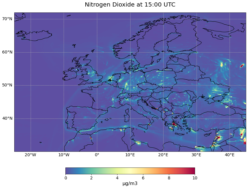
Let us now visualize the Total Column Nitrogen Dioxide information at 15:00 UTC on 7 August 2021 with the pre-defined function visualize_pcolormesh.
hour = 15
visualize_pcolormesh(data_array=no2_tc.isel(time=hour),
                     longitude=no2_tc.longitude,
                     latitude=no2_tc.latitude,
                     projection=ccrs.PlateCarree(),
                     color_scale='Spectral_r',
                     unit= no2_conc.units,
                     long_name= no2_conc.species + ' at ' + str(hour) + ':00 UTC',
                     vmin=0,
                     vmax=10,
                     lonmin=no2_tc.longitude.min(),
                     lonmax=no2_tc.longitude.max(),
                     latmin=no2_tc.latitude.min(),
                     latmax=no2_tc.latitude.max(),
                     set_global=False)
(<Figure size 1440x720 with 2 Axes>,
 <GeoAxesSubplot:title={'center':'Nitrogen Dioxide at 15:00 UTC'}>)
Copernicus ERA-5 climate reanalysis
[OPTIONAL] The second step is now to download cloud cover information from the ERA5 climate reanalysis data for the same day, 7 August 2021 from the Copernicus Climate Data Store. This step is optional because we have already downloaded the data for you, which is why the following code is commented out. The retrieve request below downloads the following data:
Date: 7 August 2021
Variable: Total Cloud Cover
Type: Reanalysis
Spatial resolution: 0.25 deg x 0.25 deg
Temporal resolution: hourly
Format: netcdf
The data is downloaded with the filename 20210807_era5_tcc.nc.
Note: Replace the hashes with your CDS credentials. You can find them here, once you are logged in.
# cds_url = '##############################'
# cds_key = '#################################'
'''
c = cdsapi.Client(url=cds_url, key=cds_key)

c.retrieve(
    'reanalysis-era5-single-levels',
    {
        'product_type': 'reanalysis',
        'variable': 'total_cloud_cover',
        'year': '2021',
        'month': '08',
        'day': '07',
        'time': [
            '00:00', '01:00', '02:00',
            '03:00', '04:00', '05:00',
            '06:00', '07:00', '08:00',
            '09:00', '10:00', '11:00',
            '12:00', '13:00', '14:00',
            '15:00', '16:00', '17:00',
            '18:00', '19:00', '20:00',
            '21:00', '22:00', '23:00',
        ],
        'area': [
            70, -25, 30,
            45,
        ],
        'format': 'netcdf',
    },
    './20210807_era5_tcc.nc')
'''
"\nc = cdsapi.Client(url=cds_url, key=cds_key)\n\nc.retrieve(\n 'reanalysis-era5-single-levels',\n {\n 'product_type': 'reanalysis',\n 'variable': 'total_cloud_cover',\n 'year': '2021',\n 'month': '08',\n 'day': '07',\n 'time': [\n '00:00', '01:00', '02:00',\n '03:00', '04:00', '05:00',\n '06:00', '07:00', '08:00',\n '09:00', '10:00', '11:00',\n '12:00', '13:00', '14:00',\n '15:00', '16:00', '17:00',\n '18:00', '19:00', '20:00',\n '21:00', '22:00', '23:00',\n ],\n 'area': [\n 70, -25, 30,\n 45,\n ],\n 'format': 'netcdf',\n },\n './20210807_era5_tcc.nc')\n"
Load and browse ERA-5 climate reanalysis data
The next step is to open the NetCDF file as xarray Dataset. You can use the function open_dataset() to open a single NetCDF file. The dataset has three dimensions (longitude, latitude and time).
file_cloud_cover = xr.open_dataset('../data/cams/2021/20210807_era5_tcc.nc')
file_cloud_cover
<xarray.Dataset>
Dimensions:    (longitude: 281, latitude: 161, time: 24)
Coordinates:
  * longitude  (longitude) float32 -25.0 -24.75 -24.5 -24.25 ... 44.5 44.75 45.0
  * latitude   (latitude) float32 70.0 69.75 69.5 69.25 ... 30.5 30.25 30.0
  * time       (time) datetime64[ns] 2021-08-07 ... 2021-08-07T23:00:00
Data variables:
    tcc        (time, latitude, longitude) float32 ...
Attributes:
    Conventions:  CF-1.6
history: 2022-02-02 16:14:14 GMT by grib_to_netcdf-2.23.0: /opt/ecmw...- longitude: 281
- latitude: 161
- time: 24
- longitude(longitude)float32-25.0 -24.75 -24.5 ... 44.75 45.0
- units :
- degrees_east
- long_name :
- longitude
array([-25. , -24.75, -24.5 , ..., 44.5 , 44.75, 45. ], dtype=float32)
- latitude(latitude)float3270.0 69.75 69.5 ... 30.5 30.25 30.0
- units :
- degrees_north
- long_name :
- latitude
array([70. , 69.75, 69.5 , 69.25, 69. , 68.75, 68.5 , 68.25, 68. , 67.75, 67.5 , 67.25, 67. , 66.75, 66.5 , 66.25, 66. , 65.75, 65.5 , 65.25, 65. , 64.75, 64.5 , 64.25, 64. , 63.75, 63.5 , 63.25, 63. , 62.75, 62.5 , 62.25, 62. , 61.75, 61.5 , 61.25, 61. , 60.75, 60.5 , 60.25, 60. , 59.75, 59.5 , 59.25, 59. , 58.75, 58.5 , 58.25, 58. , 57.75, 57.5 , 57.25, 57. , 56.75, 56.5 , 56.25, 56. , 55.75, 55.5 , 55.25, 55. , 54.75, 54.5 , 54.25, 54. , 53.75, 53.5 , 53.25, 53. , 52.75, 52.5 , 52.25, 52. , 51.75, 51.5 , 51.25, 51. , 50.75, 50.5 , 50.25, 50. , 49.75, 49.5 , 49.25, 49. , 48.75, 48.5 , 48.25, 48. , 47.75, 47.5 , 47.25, 47. , 46.75, 46.5 , 46.25, 46. , 45.75, 45.5 , 45.25, 45. , 44.75, 44.5 , 44.25, 44. , 43.75, 43.5 , 43.25, 43. , 42.75, 42.5 , 42.25, 42. , 41.75, 41.5 , 41.25, 41. , 40.75, 40.5 , 40.25, 40. , 39.75, 39.5 , 39.25, 39. , 38.75, 38.5 , 38.25, 38. , 37.75, 37.5 , 37.25, 37. , 36.75, 36.5 , 36.25, 36. , 35.75, 35.5 , 35.25, 35. , 34.75, 34.5 , 34.25, 34. , 33.75, 33.5 , 33.25, 33. , 32.75, 32.5 , 32.25, 32. , 31.75, 31.5 , 31.25, 31. , 30.75, 30.5 , 30.25, 30. ], dtype=float32) - time(time)datetime64[ns]2021-08-07 ... 2021-08-07T23:00:00
- long_name :
- time
array(['2021-08-07T00:00:00.000000000', '2021-08-07T01:00:00.000000000',
       '2021-08-07T02:00:00.000000000', '2021-08-07T03:00:00.000000000',
       '2021-08-07T04:00:00.000000000', '2021-08-07T05:00:00.000000000',
       '2021-08-07T06:00:00.000000000', '2021-08-07T07:00:00.000000000',
       '2021-08-07T08:00:00.000000000', '2021-08-07T09:00:00.000000000',
       '2021-08-07T10:00:00.000000000', '2021-08-07T11:00:00.000000000',
       '2021-08-07T12:00:00.000000000', '2021-08-07T13:00:00.000000000',
       '2021-08-07T14:00:00.000000000', '2021-08-07T15:00:00.000000000',
       '2021-08-07T16:00:00.000000000', '2021-08-07T17:00:00.000000000',
       '2021-08-07T18:00:00.000000000', '2021-08-07T19:00:00.000000000',
       '2021-08-07T20:00:00.000000000', '2021-08-07T21:00:00.000000000',
       '2021-08-07T22:00:00.000000000', '2021-08-07T23:00:00.000000000'],
      dtype='datetime64[ns]')
- tcc(time, latitude, longitude)float32...
- units :
- (0 - 1)
- long_name :
- Total cloud cover
- standard_name :
- cloud_area_fraction
[1085784 values with dtype=float32]
- Conventions :
- CF-1.6
- history :
- 2022-02-02 16:14:14 GMT by grib_to_netcdf-2.23.0: /opt/ecmwf/mars-client/bin/grib_to_netcdf -S param -o /cache/data9/adaptor.mars.internal-1643818453.9516797-27525-14-92ea8774-273f-44a9-b144-b7081246c08d.nc /cache/tmp/92ea8774-273f-44a9-b144-b7081246c08d-adaptor.mars.internal-1643818450.7729998-27525-14-tmp.grib
Now, we can load the variable tcc from the xarray Dataset. You simply specify the name of the variable and bring it into square brackets. The loaded xarray.DataArray offers additional variable attributes, e.g. units, long_name and standard_name.
cloud_cover = file_cloud_cover['tcc']
cloud_cover
<xarray.DataArray 'tcc' (time: 24, latitude: 161, longitude: 281)>
[1085784 values with dtype=float32]
Coordinates:
  * longitude  (longitude) float32 -25.0 -24.75 -24.5 -24.25 ... 44.5 44.75 45.0
  * latitude   (latitude) float32 70.0 69.75 69.5 69.25 ... 30.5 30.25 30.0
  * time       (time) datetime64[ns] 2021-08-07 ... 2021-08-07T23:00:00
Attributes:
    units:          (0 - 1)
    long_name:      Total cloud cover
standard_name: cloud_area_fraction- time: 24
- latitude: 161
- longitude: 281
- ...
[1085784 values with dtype=float32]
- longitude(longitude)float32-25.0 -24.75 -24.5 ... 44.75 45.0
- units :
- degrees_east
- long_name :
- longitude
array([-25. , -24.75, -24.5 , ..., 44.5 , 44.75, 45. ], dtype=float32)
- latitude(latitude)float3270.0 69.75 69.5 ... 30.5 30.25 30.0
- units :
- degrees_north
- long_name :
- latitude
array([70. , 69.75, 69.5 , 69.25, 69. , 68.75, 68.5 , 68.25, 68. , 67.75, 67.5 , 67.25, 67. , 66.75, 66.5 , 66.25, 66. , 65.75, 65.5 , 65.25, 65. , 64.75, 64.5 , 64.25, 64. , 63.75, 63.5 , 63.25, 63. , 62.75, 62.5 , 62.25, 62. , 61.75, 61.5 , 61.25, 61. , 60.75, 60.5 , 60.25, 60. , 59.75, 59.5 , 59.25, 59. , 58.75, 58.5 , 58.25, 58. , 57.75, 57.5 , 57.25, 57. , 56.75, 56.5 , 56.25, 56. , 55.75, 55.5 , 55.25, 55. , 54.75, 54.5 , 54.25, 54. , 53.75, 53.5 , 53.25, 53. , 52.75, 52.5 , 52.25, 52. , 51.75, 51.5 , 51.25, 51. , 50.75, 50.5 , 50.25, 50. , 49.75, 49.5 , 49.25, 49. , 48.75, 48.5 , 48.25, 48. , 47.75, 47.5 , 47.25, 47. , 46.75, 46.5 , 46.25, 46. , 45.75, 45.5 , 45.25, 45. , 44.75, 44.5 , 44.25, 44. , 43.75, 43.5 , 43.25, 43. , 42.75, 42.5 , 42.25, 42. , 41.75, 41.5 , 41.25, 41. , 40.75, 40.5 , 40.25, 40. , 39.75, 39.5 , 39.25, 39. , 38.75, 38.5 , 38.25, 38. , 37.75, 37.5 , 37.25, 37. , 36.75, 36.5 , 36.25, 36. , 35.75, 35.5 , 35.25, 35. , 34.75, 34.5 , 34.25, 34. , 33.75, 33.5 , 33.25, 33. , 32.75, 32.5 , 32.25, 32. , 31.75, 31.5 , 31.25, 31. , 30.75, 30.5 , 30.25, 30. ], dtype=float32) - time(time)datetime64[ns]2021-08-07 ... 2021-08-07T23:00:00
- long_name :
- time
array(['2021-08-07T00:00:00.000000000', '2021-08-07T01:00:00.000000000',
       '2021-08-07T02:00:00.000000000', '2021-08-07T03:00:00.000000000',
       '2021-08-07T04:00:00.000000000', '2021-08-07T05:00:00.000000000',
       '2021-08-07T06:00:00.000000000', '2021-08-07T07:00:00.000000000',
       '2021-08-07T08:00:00.000000000', '2021-08-07T09:00:00.000000000',
       '2021-08-07T10:00:00.000000000', '2021-08-07T11:00:00.000000000',
       '2021-08-07T12:00:00.000000000', '2021-08-07T13:00:00.000000000',
       '2021-08-07T14:00:00.000000000', '2021-08-07T15:00:00.000000000',
       '2021-08-07T16:00:00.000000000', '2021-08-07T17:00:00.000000000',
       '2021-08-07T18:00:00.000000000', '2021-08-07T19:00:00.000000000',
       '2021-08-07T20:00:00.000000000', '2021-08-07T21:00:00.000000000',
       '2021-08-07T22:00:00.000000000', '2021-08-07T23:00:00.000000000'],
      dtype='datetime64[ns]')
- units :
- (0 - 1)
- long_name :
- Total cloud cover
- standard_name :
- cloud_area_fraction
Interpolate ERA-5 data to a spatial resolution of CAMS European air quality forecasts
In a next step, we have to bring both datasets onto the same spatial resolution. For this reason, we resample the ERA5 reanalysis data to the spatial resolution of the CAMS European air quality forecasts, which is 0.1 deg x 0.1 deg.
You can use the function interp() to resample the coordinate of a DataArray. As target latitude and longitude information, you can provide the coordinates from the CAMS data.
cloud_cover_10km = cloud_cover.interp(latitude=no2_conc["latitude"], longitude=no2_conc["longitude"])
cloud_cover_10km
<xarray.DataArray 'tcc' (time: 24, latitude: 420, longitude: 700)>
array([[[       nan,        nan,        nan, ...,        nan,
                nan,        nan],
        [       nan,        nan,        nan, ...,        nan,
                nan,        nan],
        [       nan,        nan,        nan, ...,        nan,
                nan,        nan],
        ...,
        [0.16818032, 0.27308804, 0.3779317 , ..., 0.2933331 ,
         0.23000237, 0.1666813 ],
        [0.28166866, 0.36615285, 0.45058548, ..., 0.47645378,
         0.40946785, 0.34249216],
        [0.39515704, 0.45921767, 0.52323925, ..., 0.65957445,
         0.58893335, 0.518303  ]],

       [[       nan,        nan,        nan, ...,        nan,
                nan,        nan],
        [       nan,        nan,        nan, ...,        nan,
                nan,        nan],
        [       nan,        nan,        nan, ...,        nan,
                nan,        nan],
...
        [0.13331224, 0.13936943, 0.1454229 , ..., 0.23830742,
         0.36562204, 0.4929172 ],
        [0.13315088, 0.14110826, 0.14906079, ..., 0.27876353,
         0.41604507, 0.5533057 ],
        [0.13298951, 0.14284709, 0.15269865, ..., 0.31921965,
         0.4664681 , 0.6136941 ]],

       [[       nan,        nan,        nan, ...,        nan,
                nan,        nan],
        [       nan,        nan,        nan, ...,        nan,
                nan,        nan],
        [       nan,        nan,        nan, ...,        nan,
                nan,        nan],
        ...,
        [0.22098069, 0.20511723, 0.18926343, ..., 0.22686279,
         0.34493572, 0.4629906 ],
        [0.1823511 , 0.17435712, 0.16636801, ..., 0.2435018 ,
         0.36259046, 0.48166096],
        [0.1437215 , 0.143597  , 0.14347258, ..., 0.2601408 ,
         0.3802452 , 0.5003313 ]]], dtype=float32)
Coordinates:
  * time       (time) datetime64[ns] 2021-08-07 ... 2021-08-07T23:00:00
  * latitude   (latitude) float32 71.95 71.85 71.75 71.65 ... 30.25 30.15 30.05
  * longitude  (longitude) float32 -24.95 -24.85 -24.75 ... 44.75 44.85 44.95
Attributes:
    units:          (0 - 1)
    long_name:      Total cloud cover
standard_name: cloud_area_fraction- time: 24
- latitude: 420
- longitude: 700
- nan nan nan nan nan nan ... 0.1463 0.1798 0.22 0.2601 0.3802 0.5003
array([[[ nan, nan, nan, ..., nan, nan, nan], [ nan, nan, nan, ..., nan, nan, nan], [ nan, nan, nan, ..., nan, nan, nan], ..., [0.16818032, 0.27308804, 0.3779317 , ..., 0.2933331 , 0.23000237, 0.1666813 ], [0.28166866, 0.36615285, 0.45058548, ..., 0.47645378, 0.40946785, 0.34249216], [0.39515704, 0.45921767, 0.52323925, ..., 0.65957445, 0.58893335, 0.518303 ]], [[ nan, nan, nan, ..., nan, nan, nan], [ nan, nan, nan, ..., nan, nan, nan], [ nan, nan, nan, ..., nan, nan, nan], ... [0.13331224, 0.13936943, 0.1454229 , ..., 0.23830742, 0.36562204, 0.4929172 ], [0.13315088, 0.14110826, 0.14906079, ..., 0.27876353, 0.41604507, 0.5533057 ], [0.13298951, 0.14284709, 0.15269865, ..., 0.31921965, 0.4664681 , 0.6136941 ]], [[ nan, nan, nan, ..., nan, nan, nan], [ nan, nan, nan, ..., nan, nan, nan], [ nan, nan, nan, ..., nan, nan, nan], ..., [0.22098069, 0.20511723, 0.18926343, ..., 0.22686279, 0.34493572, 0.4629906 ], [0.1823511 , 0.17435712, 0.16636801, ..., 0.2435018 , 0.36259046, 0.48166096], [0.1437215 , 0.143597 , 0.14347258, ..., 0.2601408 , 0.3802452 , 0.5003313 ]]], dtype=float32) - time(time)datetime64[ns]2021-08-07 ... 2021-08-07T23:00:00
- long_name :
- time
array(['2021-08-07T00:00:00.000000000', '2021-08-07T01:00:00.000000000', '2021-08-07T02:00:00.000000000', '2021-08-07T03:00:00.000000000', '2021-08-07T04:00:00.000000000', '2021-08-07T05:00:00.000000000', '2021-08-07T06:00:00.000000000', '2021-08-07T07:00:00.000000000', '2021-08-07T08:00:00.000000000', '2021-08-07T09:00:00.000000000', '2021-08-07T10:00:00.000000000', '2021-08-07T11:00:00.000000000', '2021-08-07T12:00:00.000000000', '2021-08-07T13:00:00.000000000', '2021-08-07T14:00:00.000000000', '2021-08-07T15:00:00.000000000', '2021-08-07T16:00:00.000000000', '2021-08-07T17:00:00.000000000', '2021-08-07T18:00:00.000000000', '2021-08-07T19:00:00.000000000', '2021-08-07T20:00:00.000000000', '2021-08-07T21:00:00.000000000', '2021-08-07T22:00:00.000000000', '2021-08-07T23:00:00.000000000'], dtype='datetime64[ns]') - latitude(latitude)float3271.95 71.85 71.75 ... 30.15 30.05
- long_name :
- latitude
- units :
- degrees_north
array([71.95, 71.85, 71.75, ..., 30.25, 30.15, 30.05], dtype=float32)
- longitude(longitude)float32-24.95 -24.85 ... 44.85 44.95
array([-24.950012, -24.849976, -24.75    , ...,  44.75    ,  44.850006,
        44.949997], dtype=float32)
- units :
- (0 - 1)
- long_name :
- Total cloud cover
- standard_name :
- cloud_area_fraction
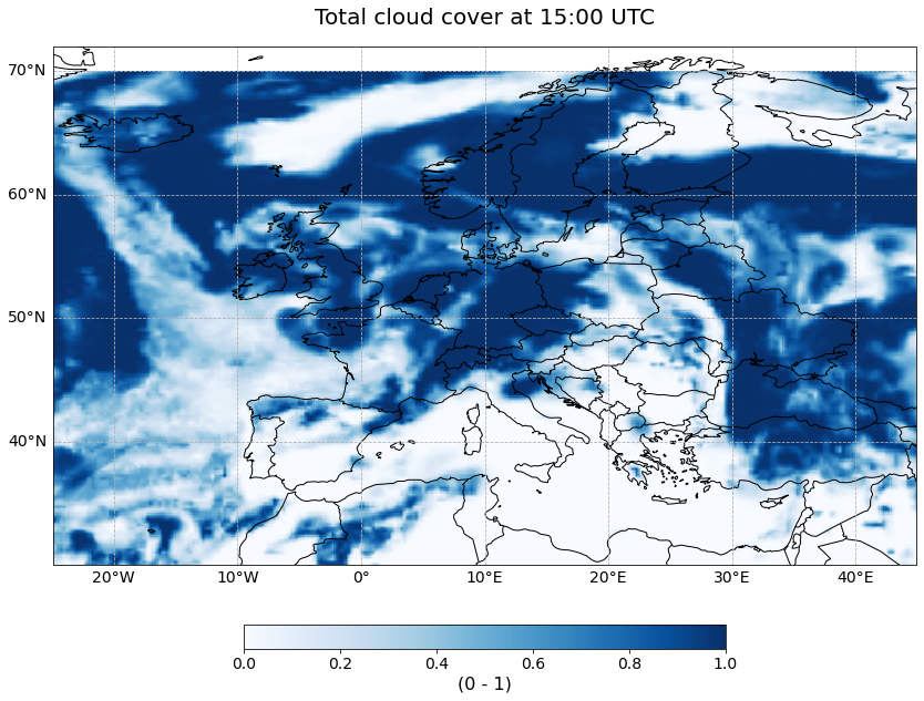
Now, we can also visualize the interpolated total cloud cover for one time step. You can use again the pre-defined function visualize_pcolormesh.
hour = 15
visualize_pcolormesh(data_array=cloud_cover_10km.isel(time=hour),
                     longitude=cloud_cover_10km.longitude,
                     latitude=cloud_cover_10km.latitude,
                     projection=ccrs.PlateCarree(),
                     color_scale='Blues',
                     unit= cloud_cover.units,
                     long_name= cloud_cover_10km.long_name + ' at ' + str(hour) + ':00 UTC',
                     vmin=0,
                     vmax=1,
                     lonmin=cloud_cover_10km.longitude.min(),
                     lonmax=cloud_cover_10km.longitude.max(),
                     latmin=cloud_cover_10km.latitude.min(),
                     latmax=cloud_cover_10km.latitude.max(),
                     set_global=False)
(<Figure size 1440x720 with 2 Axes>,
 <GeoAxesSubplot:title={'center':'Total cloud cover at 15:00 UTC'}>)
Cloud masking
Based on the total cloud cover information, we want to filter pixels with a cloud cover less than 20%. With the function where, we create below a cloud mask, asigning 1 to pixels with a cloud cover less than 20%.
cloud_mask = xr.where(cloud_cover_10km < 0.2, 1, 0)
cloud_mask
<xarray.DataArray 'tcc' (time: 24, latitude: 420, longitude: 700)>
array([[[0, 0, 0, ..., 0, 0, 0],
        [0, 0, 0, ..., 0, 0, 0],
        [0, 0, 0, ..., 0, 0, 0],
        ...,
        [1, 0, 0, ..., 0, 0, 1],
        [0, 0, 0, ..., 0, 0, 0],
        [0, 0, 0, ..., 0, 0, 0]],

       [[0, 0, 0, ..., 0, 0, 0],
        [0, 0, 0, ..., 0, 0, 0],
        [0, 0, 0, ..., 0, 0, 0],
        ...,
        [1, 0, 0, ..., 0, 0, 0],
        [0, 0, 0, ..., 0, 0, 0],
        [0, 0, 0, ..., 0, 0, 0]],

       [[0, 0, 0, ..., 0, 0, 0],
        [0, 0, 0, ..., 0, 0, 0],
        [0, 0, 0, ..., 0, 0, 0],
        ...,
...
        ...,
        [1, 1, 1, ..., 0, 0, 0],
        [1, 1, 1, ..., 0, 0, 0],
        [1, 1, 1, ..., 0, 0, 0]],

       [[0, 0, 0, ..., 0, 0, 0],
        [0, 0, 0, ..., 0, 0, 0],
        [0, 0, 0, ..., 0, 0, 0],
        ...,
        [1, 1, 1, ..., 0, 0, 0],
        [1, 1, 1, ..., 0, 0, 0],
        [1, 1, 1, ..., 0, 0, 0]],

       [[0, 0, 0, ..., 0, 0, 0],
        [0, 0, 0, ..., 0, 0, 0],
        [0, 0, 0, ..., 0, 0, 0],
        ...,
        [0, 0, 1, ..., 0, 0, 0],
        [1, 1, 1, ..., 0, 0, 0],
        [1, 1, 1, ..., 0, 0, 0]]])
Coordinates:
  * time       (time) datetime64[ns] 2021-08-07 ... 2021-08-07T23:00:00
  * latitude   (latitude) float32 71.95 71.85 71.75 71.65 ... 30.25 30.15 30.05
* longitude (longitude) float32 -24.95 -24.85 -24.75 ... 44.75 44.85 44.95- time: 24
- latitude: 420
- longitude: 700
- 0 0 0 0 0 0 0 0 0 0 0 0 0 0 0 0 0 ... 1 1 1 1 1 1 1 1 1 1 1 1 0 0 0 0
array([[[0, 0, 0, ..., 0, 0, 0], [0, 0, 0, ..., 0, 0, 0], [0, 0, 0, ..., 0, 0, 0], ..., [1, 0, 0, ..., 0, 0, 1], [0, 0, 0, ..., 0, 0, 0], [0, 0, 0, ..., 0, 0, 0]], [[0, 0, 0, ..., 0, 0, 0], [0, 0, 0, ..., 0, 0, 0], [0, 0, 0, ..., 0, 0, 0], ..., [1, 0, 0, ..., 0, 0, 0], [0, 0, 0, ..., 0, 0, 0], [0, 0, 0, ..., 0, 0, 0]], [[0, 0, 0, ..., 0, 0, 0], [0, 0, 0, ..., 0, 0, 0], [0, 0, 0, ..., 0, 0, 0], ..., ... ..., [1, 1, 1, ..., 0, 0, 0], [1, 1, 1, ..., 0, 0, 0], [1, 1, 1, ..., 0, 0, 0]], [[0, 0, 0, ..., 0, 0, 0], [0, 0, 0, ..., 0, 0, 0], [0, 0, 0, ..., 0, 0, 0], ..., [1, 1, 1, ..., 0, 0, 0], [1, 1, 1, ..., 0, 0, 0], [1, 1, 1, ..., 0, 0, 0]], [[0, 0, 0, ..., 0, 0, 0], [0, 0, 0, ..., 0, 0, 0], [0, 0, 0, ..., 0, 0, 0], ..., [0, 0, 1, ..., 0, 0, 0], [1, 1, 1, ..., 0, 0, 0], [1, 1, 1, ..., 0, 0, 0]]]) - time(time)datetime64[ns]2021-08-07 ... 2021-08-07T23:00:00
- long_name :
- time
array(['2021-08-07T00:00:00.000000000', '2021-08-07T01:00:00.000000000', '2021-08-07T02:00:00.000000000', '2021-08-07T03:00:00.000000000', '2021-08-07T04:00:00.000000000', '2021-08-07T05:00:00.000000000', '2021-08-07T06:00:00.000000000', '2021-08-07T07:00:00.000000000', '2021-08-07T08:00:00.000000000', '2021-08-07T09:00:00.000000000', '2021-08-07T10:00:00.000000000', '2021-08-07T11:00:00.000000000', '2021-08-07T12:00:00.000000000', '2021-08-07T13:00:00.000000000', '2021-08-07T14:00:00.000000000', '2021-08-07T15:00:00.000000000', '2021-08-07T16:00:00.000000000', '2021-08-07T17:00:00.000000000', '2021-08-07T18:00:00.000000000', '2021-08-07T19:00:00.000000000', '2021-08-07T20:00:00.000000000', '2021-08-07T21:00:00.000000000', '2021-08-07T22:00:00.000000000', '2021-08-07T23:00:00.000000000'], dtype='datetime64[ns]') - latitude(latitude)float3271.95 71.85 71.75 ... 30.15 30.05
- long_name :
- latitude
- units :
- degrees_north
array([71.95, 71.85, 71.75, ..., 30.25, 30.15, 30.05], dtype=float32)
- longitude(longitude)float32-24.95 -24.85 ... 44.85 44.95
array([-24.950012, -24.849976, -24.75    , ...,  44.75    ,  44.850006,
        44.949997], dtype=float32)
Time coordinates of the CAMS European air quality forecasts are in nanoseconds. We can assign the time coordinates from the ERA-5 reanalysis data, which have a datetime format. This allows us to use the time information in the plotting title and the information is in a readable format.
no2_tc_assign = no2_tc.assign_coords(time=cloud_mask.time)
Now you can apply the cloud mask onto the DataArray with the Nitrogen Dioxide information. This masking process creates the proxy data for the Sentinel-4 L2 NO2 product, which will only provide information for nearly cloud-free pixels.
no2_tc_masked = xr.where(cloud_mask==1, no2_tc_assign, np.nan)
no2_tc_masked
<xarray.DataArray (time: 24, latitude: 420, longitude: 700)>
array([[[       nan,        nan,        nan, ...,        nan,
                nan,        nan],
        [       nan,        nan,        nan, ...,        nan,
                nan,        nan],
        [       nan,        nan,        nan, ...,        nan,
                nan,        nan],
        ...,
        [0.03783086,        nan,        nan, ...,        nan,
                nan, 0.41327664],
        [       nan,        nan,        nan, ...,        nan,
                nan,        nan],
        [       nan,        nan,        nan, ...,        nan,
                nan,        nan]],

       [[       nan,        nan,        nan, ...,        nan,
                nan,        nan],
        [       nan,        nan,        nan, ...,        nan,
                nan,        nan],
        [       nan,        nan,        nan, ...,        nan,
                nan,        nan],
...
        [0.03395721, 0.0339658 , 0.03399318, ...,        nan,
                nan,        nan],
        [0.03400403, 0.03402226, 0.03402333, ...,        nan,
                nan,        nan],
        [0.03402333, 0.03402333, 0.03402333, ...,        nan,
                nan,        nan]],

       [[       nan,        nan,        nan, ...,        nan,
                nan,        nan],
        [       nan,        nan,        nan, ...,        nan,
                nan,        nan],
        [       nan,        nan,        nan, ...,        nan,
                nan,        nan],
        ...,
        [       nan,        nan, 0.03283677, ...,        nan,
                nan,        nan],
        [0.03238934, 0.03163483, 0.03161981, ...,        nan,
                nan,        nan],
        [0.03161981, 0.03161981, 0.03161981, ...,        nan,
                nan,        nan]]], dtype=float32)
Coordinates:
  * time       (time) datetime64[ns] 2021-08-07 ... 2021-08-07T23:00:00
  * latitude   (latitude) float32 71.95 71.85 71.75 71.65 ... 30.25 30.15 30.05
* longitude (longitude) float32 -24.95 -24.85 -24.75 ... 44.75 44.85 44.95- time: 24
- latitude: 420
- longitude: 700
- nan nan nan nan nan nan nan ... 0.148 0.1394 0.1325 nan nan nan nan
array([[[ nan, nan, nan, ..., nan, nan, nan], [ nan, nan, nan, ..., nan, nan, nan], [ nan, nan, nan, ..., nan, nan, nan], ..., [0.03783086, nan, nan, ..., nan, nan, 0.41327664], [ nan, nan, nan, ..., nan, nan, nan], [ nan, nan, nan, ..., nan, nan, nan]], [[ nan, nan, nan, ..., nan, nan, nan], [ nan, nan, nan, ..., nan, nan, nan], [ nan, nan, nan, ..., nan, nan, nan], ... [0.03395721, 0.0339658 , 0.03399318, ..., nan, nan, nan], [0.03400403, 0.03402226, 0.03402333, ..., nan, nan, nan], [0.03402333, 0.03402333, 0.03402333, ..., nan, nan, nan]], [[ nan, nan, nan, ..., nan, nan, nan], [ nan, nan, nan, ..., nan, nan, nan], [ nan, nan, nan, ..., nan, nan, nan], ..., [ nan, nan, 0.03283677, ..., nan, nan, nan], [0.03238934, 0.03163483, 0.03161981, ..., nan, nan, nan], [0.03161981, 0.03161981, 0.03161981, ..., nan, nan, nan]]], dtype=float32) - time(time)datetime64[ns]2021-08-07 ... 2021-08-07T23:00:00
array(['2021-08-07T00:00:00.000000000', '2021-08-07T01:00:00.000000000', '2021-08-07T02:00:00.000000000', '2021-08-07T03:00:00.000000000', '2021-08-07T04:00:00.000000000', '2021-08-07T05:00:00.000000000', '2021-08-07T06:00:00.000000000', '2021-08-07T07:00:00.000000000', '2021-08-07T08:00:00.000000000', '2021-08-07T09:00:00.000000000', '2021-08-07T10:00:00.000000000', '2021-08-07T11:00:00.000000000', '2021-08-07T12:00:00.000000000', '2021-08-07T13:00:00.000000000', '2021-08-07T14:00:00.000000000', '2021-08-07T15:00:00.000000000', '2021-08-07T16:00:00.000000000', '2021-08-07T17:00:00.000000000', '2021-08-07T18:00:00.000000000', '2021-08-07T19:00:00.000000000', '2021-08-07T20:00:00.000000000', '2021-08-07T21:00:00.000000000', '2021-08-07T22:00:00.000000000', '2021-08-07T23:00:00.000000000'], dtype='datetime64[ns]') - latitude(latitude)float3271.95 71.85 71.75 ... 30.15 30.05
array([71.95, 71.85, 71.75, ..., 30.25, 30.15, 30.05], dtype=float32)
- longitude(longitude)float32-24.95 -24.85 ... 44.85 44.95
array([-24.950012, -24.849976, -24.75    , ...,  44.75    ,  44.850006,
        44.949997], dtype=float32)
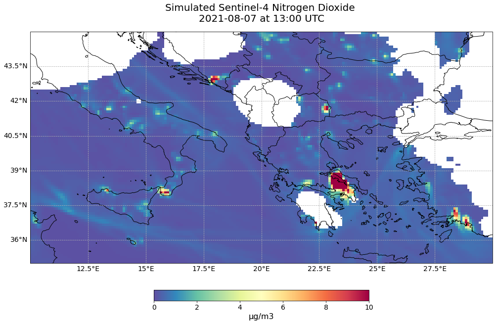
Visualize Nitrogen Dioxide on 7 August 2021 for one time step
We can now visualize the created proxy resembling Level 2 Total Column Nitrogen Dioxide data collected by the Sentinel-4 mission. You can use again the pre-defined function visualize_pcolormesh.
hour = 13
visualize_pcolormesh(data_array=no2_tc_masked.isel(time=hour),
                     longitude=no2_tc_masked.longitude,
                     latitude=no2_tc_masked.latitude,
                     projection=ccrs.PlateCarree(),
                     color_scale='Spectral_r',
                     unit= no2_conc.units,
                     long_name= 'Simulated Sentinel-4 ' + no2_conc.species + ' \n' + str(no2_tc_masked.isel(time=hour).time.data)[0:10] \
                     + ' at ' + str(no2_tc_masked.isel(time=hour).time.data)[11:16] + ' UTC',
                     vmin=0,
                     vmax=10,
                     lonmin=10,
                     lonmax=30,
                     latmin=35,
                     latmax=45,
                     set_global=False)
(<Figure size 1440x720 with 2 Axes>,
 <GeoAxesSubplot:title={'center':'Simulated Sentinel-4 Nitrogen Dioxide \n2021-08-07 at 13:00 UTC'}>)
Animate Total Column Nitrogen Dioxide over 24 hours
In the last step, you can animate the Nitrogen Dioxide over 24 hours in order to see how the trace gas developed during the 7 August 2021.
You can do animations with matplotlib’s function animation. Jupyter’s function HTML can then be used to display HTML and video content.
The animation function consists of 4 parts:
Setting the initial state:
Here, you define the general plot your animation shall use to initialise the animation. You can also define the number of frames (time steps) your animation shall have.Functions to animate:
An animation consists of three functions:draw(),init()andanimate().draw()is the function where individual frames are passed on and the figure is returned as image. In this example, the function redraws the plot for each time step.init()returns the figure you defined for the initial state.animate()returns thedraw()function and animates the function over the given number of frames (time steps).Create a
animate.FuncAnimationobject:
The functions defined before are now combined to build ananimate.FuncAnimationobject.Play the animation as video:
As a final step, you can integrate the animation into the notebook with theHTMLclass. You take the generate animation object and convert it to a HTML5 video with theto_html5_videofunction
# Setting the initial state:
# 1. Define figure for initial plot
fig, ax = visualize_pcolormesh(data_array=no2_tc_masked[0,:,:],
                               longitude=no2_tc_masked.longitude,
                               latitude=no2_tc_masked.latitude,
                               projection=ccrs.PlateCarree(),
                               color_scale='Spectral_r',
                               unit=no2_conc.units,
                               long_name= 'Simulated Sentinel-4 ' + no2_conc.species + ' \n' + str(no2_tc_masked.isel(time=0).time.data)[0:10] \
                               + ' at ' + str(no2_tc_masked.isel(time=0).time.data)[11:16] + ' UTC',
                               vmin=0,
                               vmax=10,
                               lonmin=10,
                               lonmax=30,
                               latmin=35,
                               latmax=45,
                               set_global=False)

frames = 24

def draw(i):
    img = plt.pcolormesh(no2_tc_masked.longitude,
                         no2_tc_masked.latitude,
                         no2_tc_masked[i,:,:],
                         cmap='Spectral_r',
                         transform=ccrs.PlateCarree(),
                         vmin=0,
                         vmax=10,
                         shading='auto')

    ax.set_title('Simulated Sentinel-4 ' + no2_conc.species + ' \n' + str(no2_tc_masked.isel(time=i).time.data)[0:10] + ' at ' + str(no2_tc_masked.isel(time=i).time.data)[11:16] + ' UTC', fontsize=20, pad=20.0)
    return img


def init():
    return fig


def animate(i):
    return draw(i)

ani = animation.FuncAnimation(fig, animate, frames, interval=800, blit=False,
                              init_func=init, repeat=True)

HTML(ani.to_html5_video())

# The following line which saves the video file is commented out
# ani.save('2021-08-07_S4_NO2.mp4')

plt.close(fig)
References
Generated using Copernicus Atmosphere Monitoring Service Information 2021
Hersbach, H., Bell, B., Berrisford, P., Biavati, G., Horányi, A., Muñoz Sabater, J., Nicolas, J., Peubey, C., Radu, R., Rozum, I., Schepers, D., Simmons, A., Soci, C., Dee, D., Thépaut, J-N. (2018): ERA5 hourly data on single levels from 1959 to present. Copernicus Climate Change Service (C3S) Climate Data Store (CDS). 10.24381/cds.adbb2d47
Some code in this notebook was adapted from the following source:
copyright: 2022, EUMETSAT
license: MIT
retrieved: 2022-06-28 by Sabrina Szeto
Return to the case study
Monitoring active fires with next-generation satellites: Mediterranean Fires Case Study
Nitrogen dioxide total column