.ipynb .pdf

Contents

Copernicus Atmosphere Monitoring Service (CAMS)

Global Fire Assimilation System (GFAS) data

Hint

Execute the notebook on the training platform >>

The Copernicus Atmopshere Monitoring Service (CAMS) provides consistent and quality-controlled information related to air pollution and health and greenhouse gases. CAMS data consist of global forecasts and analyses, global reanalyses, fire emissions and greenhouse gas flux inversions.

This notebook provides an introduction to the CAMS Global Fire Assimilation System (GFAS) global fire emissions data. The CAMS Global Fire Assimilation System (GFAS) assimilates fire radiative power (FRP) observations from satellite-based sensors to produce daily estimates of wildfire and biomass burning emissions. It also provides information about injection heights derived from fire observations and meteorological information from the operational weather forecasts of ECMWF.

The GFAS data output includes spatially gridded Fire Radiative Power (FRP), dry matter burnt and biomass burning emissions for a large set of chemical, greenhouse gas and aerosol species. Data are available globally on a regular latitude-longitude grid with horizontal resolution of 0.1 degrees from 2003 to present.

Basic Facts

Spatial resolution: ~10km
Spatial coverage: Global
Time step: Daily data packaged in a monthly file
Data availability: since 2003

How to access the data

CAMS GFAS data are available in either GRIB or netCDF format. They can be downloaded from the Copernicus Atmosphere Data Store (ADS). You will need to create an ADS account here.

Get more information in the CAMS GFAS data documentation.

---

Load required libraries

import os
import xarray as xr
import numpy as np
import netCDF4 as nc
import pandas as pd

# Python libraries for visualization
%matplotlib inline
import matplotlib.pyplot as plt
import matplotlib.colors
from matplotlib.cm import get_cmap
from matplotlib.axes import Axes
import cartopy
import cartopy.crs as ccrs
from cartopy.mpl.gridliner import LONGITUDE_FORMATTER, LATITUDE_FORMATTER
from cartopy.mpl.geoaxes import GeoAxes
GeoAxes._pcolormesh_patched = Axes.pcolormesh

import warnings
warnings.simplefilter(action = "ignore", category = RuntimeWarning)

Load helper functions

%run ../functions.ipynb

---

Load and browse CAMS fire emissions data

Open a CAMS GFAS netCDF file with xarray

CAMS GFAS fire emission data can be retrieved in either GRIB or NetCDF format. With the Python library xarray and the open_dataset function, we can easily read a single NetCDF file.

CAMS GFAS fire emission data are three dimensional data, with the dimensions latitude, longitude and time. The data file loaded has 31 time steps, from 1 August to 31 August 2021 and a global spatial coverage. The xarray dataset contains a data variable called frpfire.

gfas_frpfire_xr = xr.open_dataset('../data/cams/gfas/frp/2021/08/_grib2netcdf-webmars-public-svc-green-007-6fe5cac1a363ec1525f54343b6cc9fd8-cGY9R_.nc')
gfas_frpfire_xr

<xarray.Dataset>
Dimensions:    (longitude: 3600, latitude: 1800, time: 31)
Coordinates:
  * longitude  (longitude) float32 0.05 0.15 0.25 0.35 ... 359.8 359.9 360.0
  * latitude   (latitude) float32 89.95 89.85 89.75 ... -89.75 -89.85 -89.95
  * time       (time) datetime64[ns] 2021-08-01 2021-08-02 ... 2021-08-31
Data variables:
    frpfire    (time, latitude, longitude) float32 ...
Attributes:
    Conventions:  CF-1.6
    history:      2022-02-15 11:56:28 GMT by grib_to_netcdf-2.24.0: grib_to_n...

Bring longitude coordinates onto a [-180,180] grid

The longitude values are on a [0,360] grid instead of a [-180,180] grid.

You can assign new values to coordinates in an xarray.Dataset. You can do so with the assign_coords() function, which you can apply onto a xarray.Dataset. With the code below, you shift your longitude grid from [0,360] to [-180,180]. At the end, you sort the longitude values in an ascending order.

gfas_frpfire_xr_assigned = gfas_frpfire_xr.assign_coords(longitude=(((gfas_frpfire_xr.longitude + 180) % 360) - 180)).sortby('longitude')
gfas_frpfire_xr_assigned

<xarray.Dataset>
Dimensions:    (longitude: 3600, latitude: 1800, time: 31)
Coordinates:
  * longitude  (longitude) float32 -180.0 -179.9 -179.8 ... 179.8 179.9 180.0
  * latitude   (latitude) float32 89.95 89.85 89.75 ... -89.75 -89.85 -89.95
  * time       (time) datetime64[ns] 2021-08-01 2021-08-02 ... 2021-08-31
Data variables:
    frpfire    (time, latitude, longitude) float32 ...
Attributes:
    Conventions:  CF-1.6
    history:      2022-02-15 11:56:28 GMT by grib_to_netcdf-2.24.0: grib_to_n...

A quick check of the longitude coordinates of the new xarray.Dataset shows you that the longitude values range now between [-180, 180].

gfas_frpfire_xr_assigned.longitude

<xarray.DataArray 'longitude' (longitude: 3600)>
array([-179.95001, -179.85   , -179.75   , ...,  179.75   ,  179.85   ,
        179.95001], dtype=float32)
Coordinates:
  * longitude  (longitude) float32 -180.0 -179.9 -179.8 ... 179.8 179.9 180.0

We can select the data variable with [], which gives us access to the DataArray and more parameter attributes. Thus, the dataset values are wildfire radiative power and the parameter unit is W m**-2.

frpfire = gfas_frpfire_xr_assigned['frpfire']
frpfire

<xarray.DataArray 'frpfire' (time: 31, latitude: 1800, longitude: 3600)>
[200880000 values with dtype=float32]
Coordinates:
  * longitude  (longitude) float32 -180.0 -179.9 -179.8 ... 179.8 179.9 180.0
  * latitude   (latitude) float32 89.95 89.85 89.75 ... -89.75 -89.85 -89.95
  * time       (time) datetime64[ns] 2021-08-01 2021-08-02 ... 2021-08-31
Attributes:
    units:      W m**-2
    long_name:  Wildfire radiative power

Create a geographical subset for Italy and Greece

Let’s subset our data to Italy and Greece.

For geographical subsetting, you can make use of the function generate_geographical_subset. You can use ?generate_geographical_subset to open the docstring in order to see the function’s keyword arguments.

?generate_geographical_subset

Signature:
generate_geographical_subset(
    xarray,
    latmin,
    latmax,
    lonmin,
    lonmax,
    reassign=False,
)
Docstring:
Generates a geographical subset of a xarray.DataArray and if kwarg reassign=True, shifts the longitude grid 
from a 0-360 to a -180 to 180 deg grid.

Parameters:
    xarray(xarray.DataArray): a xarray DataArray with latitude and longitude coordinates
    latmin, latmax, lonmin, lonmax(int): lat/lon boundaries of the geographical subset
    reassign(boolean): default is False
    
Returns:
    Geographical subset of a xarray.DataArray.
File:      /tmp/ipykernel_8630/3979307327.py
Type:      function

You can zoom into a region by specifying a bounding box of interest. Let us set the extent to Italy and Greece with the following bounding box information:

lonmin=10
lonmax=30
latmin=35
latmax=45

Now, let us apply the function generate_geographical_subset to subset the frpfire xarray.DataArray. Let us call the new xarray.DataArray frpfire_subset.

frpfire_subset = generate_geographical_subset(xarray=frpfire, 
                                             latmin=latmin, 
                                             latmax=latmax, 
                                             lonmin=lonmin, 
                                             lonmax=lonmax)
frpfire_subset

<xarray.DataArray 'frpfire' (time: 31, latitude: 100, longitude: 200)>
array([[[0., 0., 0., ..., 0., 0., 0.],
        [0., 0., 0., ..., 0., 0., 0.],
        [0., 0., 0., ..., 0., 0., 0.],
        ...,
        [0., 0., 0., ..., 0., 0., 0.],
        [0., 0., 0., ..., 0., 0., 0.],
        [0., 0., 0., ..., 0., 0., 0.]],

       [[0., 0., 0., ..., 0., 0., 0.],
        [0., 0., 0., ..., 0., 0., 0.],
        [0., 0., 0., ..., 0., 0., 0.],
        ...,
        [0., 0., 0., ..., 0., 0., 0.],
        [0., 0., 0., ..., 0., 0., 0.],
        [0., 0., 0., ..., 0., 0., 0.]],

       [[0., 0., 0., ..., 0., 0., 0.],
        [0., 0., 0., ..., 0., 0., 0.],
        [0., 0., 0., ..., 0., 0., 0.],
        ...,
...
        ...,
        [0., 0., 0., ..., 0., 0., 0.],
        [0., 0., 0., ..., 0., 0., 0.],
        [0., 0., 0., ..., 0., 0., 0.]],

       [[0., 0., 0., ..., 0., 0., 0.],
        [0., 0., 0., ..., 0., 0., 0.],
        [0., 0., 0., ..., 0., 0., 0.],
        ...,
        [0., 0., 0., ..., 0., 0., 0.],
        [0., 0., 0., ..., 0., 0., 0.],
        [0., 0., 0., ..., 0., 0., 0.]],

       [[0., 0., 0., ..., 0., 0., 0.],
        [0., 0., 0., ..., 0., 0., 0.],
        [0., 0., 0., ..., 0., 0., 0.],
        ...,
        [0., 0., 0., ..., 0., 0., 0.],
        [0., 0., 0., ..., 0., 0., 0.],
        [0., 0., 0., ..., 0., 0., 0.]]], dtype=float32)
Coordinates:
  * longitude  (longitude) float32 10.05 10.15 10.25 10.35 ... 29.75 29.85 29.95
  * latitude   (latitude) float32 44.95 44.85 44.75 44.65 ... 35.25 35.15 35.05
  * time       (time) datetime64[ns] 2021-08-01 2021-08-02 ... 2021-08-31
Attributes:
    units:      W m**-2
    long_name:  Wildfire radiative power

Above, you see that the variable frpfire_subset has two attributes, units and long_name. Let us define variables for those attributes. The variables can be used for visualizing the data.

units = frpfire_subset.units
long_name= frpfire_subset.long_name

Visualise CAMS GFAS fire emissions data

You can use the function visualize_pcolormesh to visualize the CAMS global fire emissions data with matplotlib’s function pcolormesh.

You can make use of the data attributes units and long_name and use them for plotting.

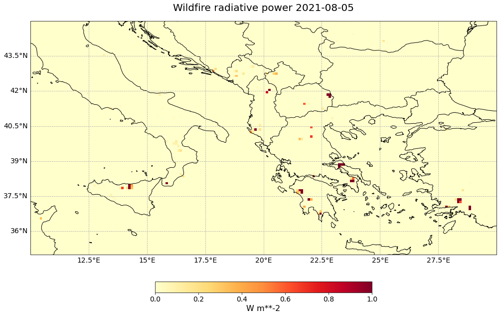
visualize_pcolormesh(data_array=frpfire_subset.isel(time=4).data,
                     longitude=frpfire_subset.longitude.data,
                     latitude=frpfire_subset.latitude.data,
                     projection=ccrs.PlateCarree(),
                     color_scale='YlOrRd',
                     unit=units,
                     long_name=long_name + ' ' + str(frpfire_subset.isel(time=4).time.data)[0:10],
                     vmin=0, 
                     vmax=1,
                     lonmin=lonmin,
                     lonmax=lonmax,
                     latmin=latmin,
                     latmax=latmax,
                     set_global=False)

(<Figure size 1440x720 with 2 Axes>,
 <GeoAxesSubplot:title={'center':'Wildfire radiative power 2021-08-05'}>)

---

References

• Kaiser, J. W., and Coauthors. (2012). Biomass burning emissions estimated with a global fire assimilation system based on observed fire radiative power, Biogeosciences, 9, 527-554, https://doi.org/10.5194/bg-9-527-2012.

• Some code in this notebook was adapted from the following source:

  • origin: https://gitlab.eumetsat.int/eumetlab/atmosphere/atmosphere/-/blob/master/20_data_exploration/262_CAMS_GFAS_FRPFIRE_load_browse.ipynb

  • copyright: 2022, EUMETSAT

  • license: MIT

  • retrieved: 2022-06-28 by Sabrina Szeto

Return to the case study

Monitoring active fires with next-generation satellites: Mediterranean Fires Case Study
Fire Radiative Power (CAMS GFAS)

previous

MODIS Level 2 - MCD14DL - Fire Radiative Power

next

Copernicus Sentinel-5P TROPOMI - Ultraviolet Aerosol Index - Level 2