.ipynb .pdf

Contents

LSA SAF Normalized Difference Vegetation Index (NDVI) - Anomaly

Hint

Execute the notebook on the training platform >>

The LSA SAF Normalized Difference Vegetation Index (NDVI) are near-global, 10-daily composite images which are synthesized from the “best available” observations registered in the course of every “dekad” by the orbiting earth observation system MetOp-AVHRR. The composites represent a Normalized Difference Vegetation Index and are distributed together with a set of ancillary dataset layers (surface reflectances, sun and view angles, quality indicators) as part of EUMETSAT LSA SAF program.

From a temporal aspect, every month is divided in three “dekads”. The first two always comprise ten days (1-10, 11-20), the third one has variable length as it runs from day 21 until the end of the month. The distinction between “days” is based on UT/GMT criteria.

From a spectral aspect, each composite comprises twelve separate image layers. The NDV layer represents the Normalized Difference Vegetation Index, while the other layers are considered as ancillary layers: synthesis reflectance values, viewing angles, status map.

The events featured in this notebook are the wildfires in Italy and Greece in summer 2021.

Basic Facts

Spatial resolution: 1km
Spatial coverage: Ten pre-defined geographical regions - see Product User Manual for more information
Time steps: Dekad (approx. 10 days)
Data availability: since 2007

How to access the data

The NDVI data can be ordered via LSA SAF.

The composites are disseminated to the users in zip archives with data from one of the ten pre-defined geographical regions. Each zip archive contains a total of 26 files: twelve IMGs, twelve HDRs, one XML (INSPIRE compatible metadata) and one TIFF (a quicklook map of the NDVI layer).

You need to register for an account before being able to download data.

---

Load required libraries

import os
import glob
import xarray as xr
import datetime
import numpy as np
import pandas as pd

# Python libraries for visualisation
from matplotlib import pyplot as plt
import cartopy.crs as ccrs
from cartopy.mpl.gridliner import LONGITUDE_FORMATTER, LATITUDE_FORMATTER
from matplotlib.colors import BoundaryNorm, ListedColormap
import cartopy.feature as cfeature

from IPython.display import display, clear_output

Load helper functions

%run ../functions.ipynb

---

Load LSA SAF NDVI image files as xarray DataArray

For this case study, we downloaded the zip archives via the LSA SAF, with the NDVI data for the Europe region of the third dekad in July for the years 2010 to 2021. On the platform, only the img files for each year are being made available and are stored in the folder ../data/lsasaf/ndvi/.

The first step is to combine all the files in a list of files and sort it based on name, to ensure the correct sequence of years.

filelist = sorted(glob.glob('../data/lsasaf/ndvi/*.img'))
filelist

['../data/lsasaf/ndvi/METOP_AVHRR_20100721_S10_EUR_NDV.img',
 '../data/lsasaf/ndvi/METOP_AVHRR_20110721_S10_EUR_NDV.img',
 '../data/lsasaf/ndvi/METOP_AVHRR_20120721_S10_EUR_NDV.img',
 '../data/lsasaf/ndvi/METOP_AVHRR_20130721_S10_EUR_NDV.img',
 '../data/lsasaf/ndvi/METOP_AVHRR_20140721_S10_EUR_NDV.img',
 '../data/lsasaf/ndvi/METOP_AVHRR_20150721_S10_EUR_NDV.img',
 '../data/lsasaf/ndvi/METOP_AVHRR_20160721_S10_EUR_NDV.img',
 '../data/lsasaf/ndvi/METOP_AVHRR_20170721_S10_EUR_NDV.img',
 '../data/lsasaf/ndvi/METOP_AVHRR_20180721_S10_EUR_NDV.img',
 '../data/lsasaf/ndvi/METOP_AVHRR_20190721_S10_EUR_NDV.img',
 '../data/lsasaf/ndvi/METOP_AVHRR_20200721_S10_EUR_NDV.img',
 '../data/lsasaf/ndvi/METOP_AVHRR_20210721_S10_EUR_NDV.img']

Define spatial and temporal coordinates

The image layers are provided in “flat binary” format without header/trailer bytes. “Flat” means that each layer of a certain composite is stored in a separate image file. These files have the fixed extension .img. Because all layers have the byte data type (1 pixel = 1 byte), the total number of bytes in each image is equal to the number of pixels. The files are disseminated in an unprojected Geographica latitude / longitude projection in WGS84. The Product User Manual provides spatial characterics, with which we are able to build the geographic latitude and longitude information:

• Resolution: 0.0089285714

• Latitude bounds: [25, 75]

• Longitude bounds: [-11, 62]

• ncols, nrows: [8176, 5600]

res = 0.0089285714

lat = np.arange(25+(res/2),75-(res/2),res)
lon = np.arange(-11+(res/2),62-(res/2),res)

print(len(lat), len(lon))

5600 8176

Since we also want to combine the NDVI value of several years, we also define a DateTimeIndex object, which holds provides for each year from 2010 to 2021 a datetime object for month July.

time_coords = pd.date_range('2010-07', '2021-07', freq='MS').strftime("%Y-%m").astype('datetime64[ns]')[::12]
time_coords

DatetimeIndex(['2010-07-01', '2011-07-01', '2012-07-01', '2013-07-01',
               '2014-07-01', '2015-07-01', '2016-07-01', '2017-07-01',
               '2018-07-01', '2019-07-01', '2020-07-01', '2021-07-01'],
              dtype='datetime64[ns]', freq=None)

data=np.fromfile(filelist[0],dtype='uint8')
data

array([255, 255, 255, ..., 255, 255, 255], dtype=uint8)

data.shape = (-1, 8176)
data.shape

(5600, 8176)

Loop through the files and combine them in a xarray DataArray

Now, you can loop through each file in the created list of files and execute the following operations:

• 1. Open the file with numpy.fromfile

• 1. Restructure the 1-dimensional array to a 2D array with 8176 columns and 5600 rows

• 1. Convert the data type to float64

• 1. Mask out the missing value and apply scale and offset

• 1. Convert the masked data array to a xarray.DataArray

• 1. Create a 3-dimensional xarray.DataArray with time and geographical coordinates as well as attributes

• 1. Flip the latitude axis

• 1. Concatenate multiple years into one xarray.DataArray

j = 0
tmp_concat=None
dtype = 'uint8'
samples=8176

for i in filelist:
    print(i)

    # 1. Open the image file
    data=np.fromfile(i,dtype=dtype)
    
    # 2. Convert to 2D array
    data.shape=(-1,samples)
    data

    # 3. Convert to float64 datatype
    data_2 = np.float64(data)
    
    # 4. Mask out the missing value and apply scale and offset
    missing_value = np.max(data)
    data_masked = np.ma.masked_values(data_2, missing_value)
    data_masked_4 = 0.004*data_masked-0.08

    # 5. Convert the masked data array to a xarray.DataArray
    xr_ds = xr.DataArray(data_masked_4)
    
    # 6. Create a 3-dimensional xarray.DataArray with time and geographical coordinates as well as attributes
    tmp = xr.DataArray(
                xr_ds.values,
                dims=['latitude','longitude'],
                coords={
                    'time': time_coords[j],
                    'latitude':(['latitude'],lat[::-1]),
                    'longitude':(['longitude'],lon)
                },
                attrs={'long_name': 'Normalized Difference Vegetation Index (ENDVI10)', 'units': '-'},
                name='NDVI'
            )
    
    # 7. Flip the latitude axis
    tmp = tmp.reindex(latitude=tmp.latitude[::-1])
    
    # 8. Concatenate multiple years into one xarray.DataArray
    if tmp_concat is None:
        tmp_concat = tmp
        
    else:
        tmp_concat = xr.concat([tmp_concat, tmp], dim='time')
    
    j = j+1

../data/lsasaf/ndvi/METOP_AVHRR_20100721_S10_EUR_NDV.img
../data/lsasaf/ndvi/METOP_AVHRR_20110721_S10_EUR_NDV.img
../data/lsasaf/ndvi/METOP_AVHRR_20120721_S10_EUR_NDV.img
../data/lsasaf/ndvi/METOP_AVHRR_20130721_S10_EUR_NDV.img
../data/lsasaf/ndvi/METOP_AVHRR_20140721_S10_EUR_NDV.img
../data/lsasaf/ndvi/METOP_AVHRR_20150721_S10_EUR_NDV.img
../data/lsasaf/ndvi/METOP_AVHRR_20160721_S10_EUR_NDV.img
../data/lsasaf/ndvi/METOP_AVHRR_20170721_S10_EUR_NDV.img
../data/lsasaf/ndvi/METOP_AVHRR_20180721_S10_EUR_NDV.img
../data/lsasaf/ndvi/METOP_AVHRR_20190721_S10_EUR_NDV.img
../data/lsasaf/ndvi/METOP_AVHRR_20200721_S10_EUR_NDV.img
../data/lsasaf/ndvi/METOP_AVHRR_20210721_S10_EUR_NDV.img

The resulting xarray object has three dimensions: time, latitude and longitude and contains for every year from 2010 to 2021 the NDVI values for the third dekad in July.

tmp_concat

<xarray.DataArray 'NDVI' (time: 12, latitude: 5600, longitude: 8176)>
array([[[0.104, 0.104, 0.104, ...,   nan,   nan,   nan],
        [0.108, 0.108, 0.108, ...,   nan,   nan,   nan],
        [0.112, 0.112, 0.108, ...,   nan,   nan,   nan],
        ...,
        [  nan,   nan,   nan, ...,   nan,   nan,   nan],
        [  nan,   nan,   nan, ...,   nan,   nan,   nan],
        [  nan,   nan,   nan, ...,   nan,   nan,   nan]],

       [[0.104, 0.104, 0.104, ...,   nan,   nan,   nan],
        [0.104, 0.104, 0.104, ...,   nan,   nan,   nan],
        [0.104, 0.104, 0.104, ...,   nan,   nan,   nan],
        ...,
        [  nan,   nan,   nan, ...,   nan,   nan,   nan],
        [  nan,   nan,   nan, ...,   nan,   nan,   nan],
        [  nan,   nan,   nan, ...,   nan,   nan,   nan]],

       [[0.1  , 0.1  , 0.096, ...,   nan,   nan,   nan],
        [0.1  , 0.1  , 0.096, ...,   nan,   nan,   nan],
        [0.104, 0.104, 0.104, ...,   nan,   nan,   nan],
        ...,
...
        ...,
        [  nan,   nan,   nan, ...,   nan,   nan,   nan],
        [  nan,   nan,   nan, ...,   nan,   nan,   nan],
        [  nan,   nan,   nan, ...,   nan,   nan,   nan]],

       [[0.092, 0.092, 0.096, ...,   nan,   nan,   nan],
        [0.096, 0.096, 0.096, ...,   nan,   nan,   nan],
        [0.1  , 0.096, 0.096, ...,   nan,   nan,   nan],
        ...,
        [  nan,   nan,   nan, ...,   nan,   nan,   nan],
        [  nan,   nan,   nan, ...,   nan,   nan,   nan],
        [  nan,   nan,   nan, ...,   nan,   nan,   nan]],

       [[0.096, 0.096, 0.092, ...,   nan,   nan,   nan],
        [0.096, 0.092, 0.092, ...,   nan,   nan,   nan],
        [0.096, 0.096, 0.096, ...,   nan,   nan,   nan],
        ...,
        [  nan,   nan,   nan, ...,   nan,   nan,   nan],
        [  nan,   nan,   nan, ...,   nan,   nan,   nan],
        [  nan,   nan,   nan, ...,   nan,   nan,   nan]]])
Coordinates:
  * latitude   (latitude) float64 25.0 25.01 25.02 25.03 ... 74.98 74.99 75.0
  * time       (time) datetime64[ns] 2010-07-01 2011-07-01 ... 2021-07-01
  * longitude  (longitude) float64 -11.0 -10.99 -10.98 ... 61.98 61.99 62.0
Attributes:
    long_name:  Normalized Difference Vegetation Index (ENDVI10)
    units:      -

Create a geographical subset for the Mediterranean region

The second step is to create a geographical subset for the Mediterranean region, with a specific focus on southern Italy and Greece (latitude bounds: 35 - 45 degrees, longitude bounds: 10 - 30 degrees). You can use the pre-defined function generate_geographical_subset to subset the xarray DataArray based on the defined extent.

The latitude points reduced from 5600 to 1120 and the longitude points reduce from 8176 to 2240, respectively.

latmin=35
latmax=45
lonmin=10
lonmax=30

ndvi_subset = generate_geographical_subset(xarray=tmp_concat,
                                           latmin=latmin,
                                           latmax=latmax,
                                           lonmin=lonmin,
                                           lonmax=lonmax
                                          )

ndvi_subset

<xarray.DataArray 'NDVI' (time: 12, latitude: 1120, longitude: 2240)>
array([[[0.176, 0.184, 0.176, ...,   nan,   nan,   nan],
        [0.192, 0.188, 0.18 , ...,   nan,   nan,   nan],
        [0.176, 0.176, 0.172, ...,   nan,   nan,   nan],
        ...,
        [0.636, 0.564, 0.592, ...,   nan,   nan,   nan],
        [0.72 , 0.712, 0.66 , ...,   nan,   nan,   nan],
        [0.744, 0.688, 0.688, ...,   nan,   nan,   nan]],

       [[0.196, 0.196, 0.188, ...,   nan,   nan,   nan],
        [0.2  , 0.188, 0.192, ...,   nan,   nan,   nan],
        [0.192, 0.192, 0.192, ...,   nan,   nan,   nan],
        ...,
        [0.716, 0.712, 0.684, ...,   nan,   nan,   nan],
        [0.716, 0.716, 0.712, ...,   nan,   nan,   nan],
        [0.708, 0.76 , 0.768, ...,   nan,   nan,   nan]],

       [[0.188, 0.196, 0.192, ...,   nan,   nan,   nan],
        [0.184, 0.18 , 0.176, ...,   nan,   nan,   nan],
        [0.184, 0.18 , 0.18 , ...,   nan,   nan,   nan],
        ...,
...
        ...,
        [0.636, 0.636, 0.516, ...,   nan,   nan,   nan],
        [0.7  , 0.62 , 0.484, ...,   nan,   nan,   nan],
        [0.648, 0.644, 0.644, ...,   nan,   nan,   nan]],

       [[0.2  , 0.196, 0.188, ...,   nan,   nan,   nan],
        [0.188, 0.184, 0.188, ...,   nan,   nan,   nan],
        [0.172, 0.16 , 0.148, ...,   nan,   nan,   nan],
        ...,
        [0.656, 0.644, 0.56 , ...,   nan,   nan,   nan],
        [0.64 , 0.628, 0.616, ...,   nan,   nan,   nan],
        [0.68 , 0.692, 0.672, ...,   nan,   nan,   nan]],

       [[0.176, 0.184, 0.172, ...,   nan,   nan,   nan],
        [0.196, 0.184, 0.152, ...,   nan,   nan,   nan],
        [0.184, 0.168, 0.16 , ...,   nan,   nan,   nan],
        ...,
        [0.6  , 0.524, 0.492, ...,   nan,   nan,   nan],
        [0.596, 0.548, 0.508, ...,   nan,   nan,   nan],
        [0.648, 0.648, 0.62 , ...,   nan,   nan,   nan]]])
Coordinates:
  * latitude   (latitude) float64 35.0 35.01 35.02 35.03 ... 44.98 44.99 45.0
  * time       (time) datetime64[ns] 2010-07-01 2011-07-01 ... 2021-07-01
  * longitude  (longitude) float64 10.0 10.01 10.02 10.03 ... 29.98 29.99 30.0
Attributes:
    long_name:  Normalized Difference Vegetation Index (ENDVI10)
    units:      -

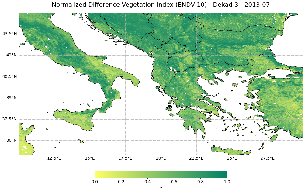
Now, you can visualize the NDVI data for one specific year. For this, you can use the pre-defined function visualize_pcolormesh, which combines matplotlib’s pcolormesh() function and the Cartopy library to visualize the data. The function takes the following keyword arguments:

• data_array: xarray DataArray to be visualized

• latitude, longitude: latitude and longitude information from the xarray

• projection: one of Cartopy’s projection options, e.g. ccrs.PlateCarree()

• color_scale: one of Matplotlib’s colormap, e.g. summer_r

• unit: unit of the data, can be used from the DataArray attributes

• long_name: description of the data, can be used from the DataArray attributes

• vmin, vmax: minimum and maximum data bounds, for NDVI it is [0,1]

• set_global: boolean; if False, then geographic extent has to be defined

• lonmin, lonmax, latmin, latmax: bounding box information to set the extent of a geographical subset

year=3

visualize_pcolormesh(data_array=ndvi_subset[year,:,:], 
                     longitude=ndvi_subset.longitude, 
                     latitude=ndvi_subset.latitude, 
                     projection=ccrs.PlateCarree(), 
                     color_scale='summer_r', 
                     unit=ndvi_subset.units, 
                     long_name=ndvi_subset.long_name + " - Dekad 3 - " + str(ndvi_subset.time[year].data)[0:7], 
                     vmin=0, 
                     vmax=1, 
                     lonmin=ndvi_subset.longitude.min(),
                     lonmax=ndvi_subset.longitude.max(),
                     latmin=ndvi_subset.latitude.min(),
                     latmax=ndvi_subset.latitude.max(),
                     set_global=False)

(<Figure size 1440x720 with 2 Axes>,
 <GeoAxesSubplot:title={'center':'Normalized Difference Vegetation Index (ENDVI10) - Dekad 3 - 2013-07'}>)

Calculate the NDVI anomaly of the third dekad of July 2021

The next step is to calculate the NDVI anomaly of the third dekad of July 2021. For this, we first calculate the average NDVI for each pixel based on a normal period of eleven years - from 2010 to 2020.

You can do this by applying the reducer function mean to the DataArray and define the dimension time by which you want to aggregate the values. The resulting array has two dimensions left, latitude and longitude and holds the average NDVI for each pixel, based on the period 2010 to 2020.

normal_period = ndvi_subset[0:11,:,:]
ndvi_mean = normal_period.mean(dim='time', keep_attrs=True)
ndvi_mean

<xarray.DataArray 'NDVI' (latitude: 1120, longitude: 2240)>
array([[0.17563636, 0.17345455, 0.16727273, ...,        nan,        nan,
               nan],
       [0.17672727, 0.16727273, 0.16145455, ...,        nan,        nan,
               nan],
       [0.17127273, 0.16290909, 0.15890909, ...,        nan,        nan,
               nan],
       ...,
       [0.64      , 0.58      , 0.54181818, ...,        nan,        nan,
               nan],
       [0.62436364, 0.60109091, 0.58872727, ...,        nan,        nan,
               nan],
       [0.66254545, 0.65527273, 0.64945455, ...,        nan,        nan,
               nan]])
Coordinates:
  * latitude   (latitude) float64 35.0 35.01 35.02 35.03 ... 44.98 44.99 45.0
  * longitude  (longitude) float64 10.0 10.01 10.02 10.03 ... 29.98 29.99 30.0
Attributes:
    long_name:  Normalized Difference Vegetation Index (ENDVI10)
    units:      -

ndvi_subset[11,:,:]

<xarray.DataArray 'NDVI' (latitude: 1120, longitude: 2240)>
array([[0.176, 0.184, 0.172, ...,   nan,   nan,   nan],
       [0.196, 0.184, 0.152, ...,   nan,   nan,   nan],
       [0.184, 0.168, 0.16 , ...,   nan,   nan,   nan],
       ...,
       [0.6  , 0.524, 0.492, ...,   nan,   nan,   nan],
       [0.596, 0.548, 0.508, ...,   nan,   nan,   nan],
       [0.648, 0.648, 0.62 , ...,   nan,   nan,   nan]])
Coordinates:
  * latitude   (latitude) float64 35.0 35.01 35.02 35.03 ... 44.98 44.99 45.0
    time       datetime64[ns] 2021-07-01
  * longitude  (longitude) float64 10.0 10.01 10.02 10.03 ... 29.98 29.99 30.0
Attributes:
    long_name:  Normalized Difference Vegetation Index (ENDVI10)
    units:      -

You can calculate the anomaly for the third dekad in July 2021 by subracting the average NDVI values from the DataArray.

ndvi_anomaly = ndvi_subset[11,:,:] - ndvi_mean
ndvi_anomaly

<xarray.DataArray 'NDVI' (latitude: 1120, longitude: 2240)>
array([[ 0.00036364,  0.01054545,  0.00472727, ...,         nan,
                nan,         nan],
       [ 0.01927273,  0.01672727, -0.00945455, ...,         nan,
                nan,         nan],
       [ 0.01272727,  0.00509091,  0.00109091, ...,         nan,
                nan,         nan],
       ...,
       [-0.04      , -0.056     , -0.04981818, ...,         nan,
                nan,         nan],
       [-0.02836364, -0.05309091, -0.08072727, ...,         nan,
                nan,         nan],
       [-0.01454545, -0.00727273, -0.02945455, ...,         nan,
                nan,         nan]])
Coordinates:
  * latitude   (latitude) float64 35.0 35.01 35.02 35.03 ... 44.98 44.99 45.0
    time       datetime64[ns] 2021-07-01
  * longitude  (longitude) float64 10.0 10.01 10.02 10.03 ... 29.98 29.99 30.0

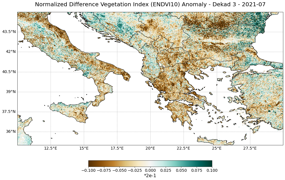
Visualize the NDVI anomaly for the third dekad in July 2021

The last step is to visualize the NDVI anomaly for the third dekad in July 2021. You can use again the function visualize_pcolormesh. Let us make some changes to some kwargs:

• data_array: now we want to visualize the ndvi_anomaly array

• color_scale: let’s use BrBG to highlight greener and less greener areas more prominently

• vmin, vmax: let us adjust the minimum and maximum color values based on the minimum and maximum anomaly values

visualize_pcolormesh(data_array=ndvi_anomaly, 
                     longitude=ndvi_anomaly.longitude, 
                     latitude=ndvi_anomaly.latitude, 
                     projection=ccrs.PlateCarree(), 
                     color_scale='BrBG', 
                     unit="*2e-1", 
                     long_name=ndvi_subset.long_name + " Anomaly - Dekad 3 - " + str(ndvi_anomaly.time.data)[0:7], 
                     vmin=-0.5*2e-1, 
                     vmax=0.5*2e-1, 
                     lonmin=ndvi_anomaly.longitude.min(),
                     lonmax=ndvi_anomaly.longitude.max(),
                     latmin=ndvi_anomaly.latitude.min(),
                     latmax=ndvi_anomaly.latitude.max(),
                     set_global=False)

(<Figure size 1440x720 with 2 Axes>,
 <GeoAxesSubplot:title={'center':'Normalized Difference Vegetation Index (ENDVI10) Anomaly - Dekad 3 - 2021-07'}>)

---

References

• Trigo, I. F., C. C. DaCamara, P. Viterbo, J.-L. Roujean, F. Olesen, C. Barroso, F. Camacho-de Coca, D. Carrer, S. C. Freitas, J. García-Haro, B. Geiger, F. Gellens-Meulenberghs, N. Ghilain, J. Meliá, L. Pessanha, N. Siljamo, and A. Arboleda. (2011). The Satellite Application Facility on Land Surface Analysis. Int. J. Remote Sens., 32, 2725-2744, doi: 10.1080/01431161003743199

• Some code in this notebook was adapted from the following source:

  • origin: https://stackoverflow.com/questions/53643062/lsa-saf-satellite-hdf5-plot-in-python-cartopy

  • copyright: 2018, methane rain

  • license: CC BY-SA 4.0

  • retrieved: 2022-06-28 by Sabrina Szeto

Return to the case study

Assessing pre-fire risk with next-generation satellites: Mediterranean Fires Case Study
Normalised Difference Vegetation Index (NDVI)

previous

Forecasting pre-fire risk with next-generation satellites

next

LSA SAF Fire Risk Map v2