MODIS Level 2 - MCD14DL - Fire Radiative Power¶

Hint

Execute the notebook on the training platform >>

This notebook provides you an introduction to data from the Moderate Resolution Imaging Spectroradiometer (MODIS). We are using MODIS fire radiative power data as a proxy for the next-generation Fire Radiative Power Pixel (FRPPIXEL) product from LSA SAF that will integrate data from Meteosat Third Generation’s Flexible Combined Imager.

This notebook shows the structure of MODIS Thermal Anomalies/Fire locations 1km FIRMS V0061 NRT (Vector data) and how to load, browse and visualize the data.

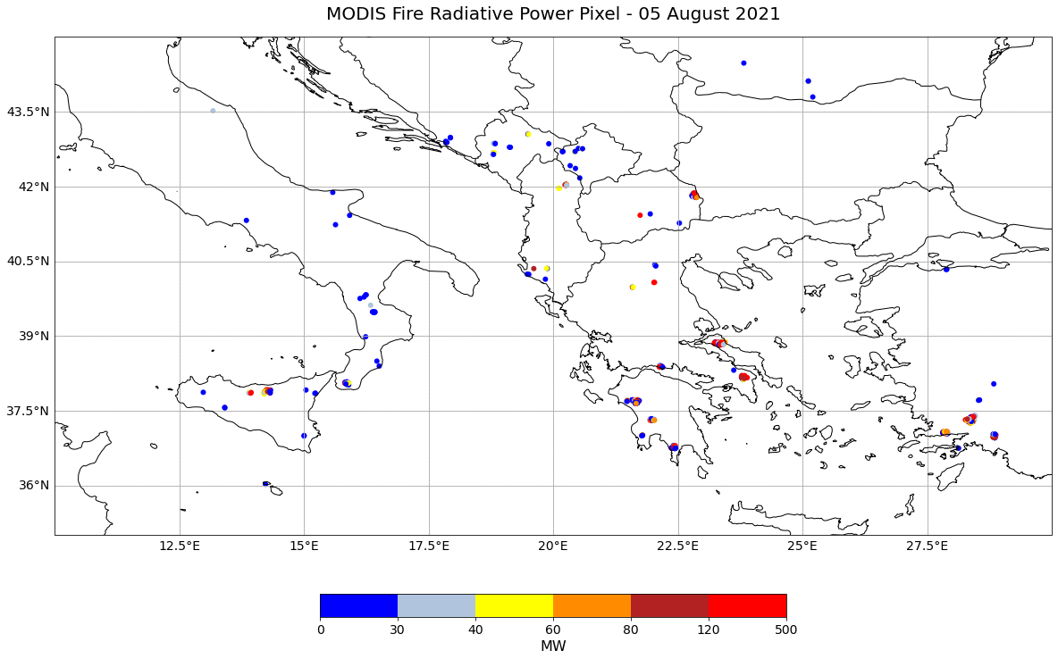
The events featured in this notebook are the wildfires in Italy and Greece in summer 2021.

Basic Facts

Spatial coverage: Global
Time step: Monthly
Data availability: since 2000

How to access the data

This notebook uses the MODIS MCD14DL dataset from the Terra and Aqua platforms. The MCD14DL dataset archive can be ordered via the FIRMS and are distributed in shp, kml or csv format, which is then zipped.

You need to register for an Earthdata account before being able to download data.

Load required libraries

import os
import numpy as np
import pandas as pd

# Python libraries for visualization
import matplotlib.colors
from matplotlib.colors import BoundaryNorm, ListedColormap
import matplotlib.pyplot as plt
import cartopy
import cartopy.crs as ccrs
from cartopy.mpl.gridliner import LONGITUDE_FORMATTER, LATITUDE_FORMATTER
from matplotlib.axes import Axes
from cartopy.mpl.geoaxes import GeoAxes
GeoAxes._pcolormesh_patched = Axes.pcolormesh

import warnings
warnings.filterwarnings('ignore')
warnings.simplefilter(action = "ignore", category = RuntimeWarning)

Load helper functions

%run ../functions.ipynb

Load and browse MODIS Fire Radiative Power data¶

[OPTIONAL] The first step is to unzip file from the zipped archive downloaded. This is optional as we have already unzipped the file for you. This is why the code is commented out.

The zipped archive contains data in a Comma-Separated Values or csv file and a Readme text document. The period requested was from 5 August 2021 to 7 August 2021.

# import zipfile
# with zipfile.ZipFile('../data/modis/level2/frp/DL_FIRE_M-C61_251212.zip', 'r') as zip_ref:
#    zip_ref.extractall('../data/modis/level2/frp/2021/08')

After we downloaded the station observations as a csv file, we can open it with the pandas function read_table(). We additonally set specific keyword arguments that allow us to specify the columns and rows of interest:

delimiter: specify the delimiter in the text file, e.g. comma
header: specify the index of the row that shall be set as header.
index_col: specify the index of the column that shall be set as index

You see below that the resulting dataframe has 2108 rows and 14 columns.

df = pd.read_table('../data/modis/level2/frp/2021/08/fire_archive_M-C61_251212.csv', delimiter=',', header=[0], index_col=5)
df

	latitude	longitude	brightness	scan	track	acq_time	satellite	instrument	confidence	version	bright_t31	frp	daynight	type
acq_date
2021-08-05	44.1170	25.1176	311.1	1.0	1.0	26	Aqua	MODIS	82	6.03	287.8	11.6	N	0
2021-08-05	42.0245	20.2539	300.0	1.3	1.1	26	Aqua	MODIS	2	6.03	289.6	4.4	N	0
2021-08-05	42.0330	20.2704	308.4	1.3	1.1	26	Aqua	MODIS	74	6.03	291.1	11.4	N	0
2021-08-05	42.0345	20.2566	353.5	1.3	1.1	26	Aqua	MODIS	100	6.03	295.1	101.7	N	0
2021-08-05	42.0362	20.2410	325.0	1.3	1.1	26	Aqua	MODIS	100	6.03	291.2	32.3	N	0
...	...	...	...	...	...	...	...	...	...	...	...	...	...	...
2021-08-07	44.7821	20.5855	326.8	1.1	1.1	2043	Terra	MODIS	100	6.03	292.9	29.1	N	0
2021-08-07	44.7837	20.5996	362.9	1.1	1.1	2043	Terra	MODIS	100	6.03	297.5	110.4	N	0
2021-08-07	43.2199	12.6086	306.7	1.5	1.2	2043	Terra	MODIS	69	6.03	293.5	10.7	N	0
2021-08-07	37.0451	28.8563	302.3	3.6	1.8	2320	Aqua	MODIS	38	6.03	290.5	32.9	N	0
2021-08-07	37.0504	28.8543	308.4	3.6	1.8	2320	Aqua	MODIS	74	6.03	290.3	56.2	N	0

2108 rows × 14 columns

From the dataframe above, let us only select the columns of interest for us. This makes the handling of the dataframe much easier. The columns of interest are: acq_date, latitude, longitude, confidence and frp. You can use the function filter() to select specific columns.

frp = df.filter(['acq_date','latitude','longitude','confidence','frp'])
frp

	latitude	longitude	confidence	frp
acq_date
2021-08-05	44.1170	25.1176	82	11.6
2021-08-05	42.0245	20.2539	2	4.4
2021-08-05	42.0330	20.2704	74	11.4
2021-08-05	42.0345	20.2566	100	101.7
2021-08-05	42.0362	20.2410	100	32.3
...	...	...	...	...
2021-08-07	44.7821	20.5855	100	29.1
2021-08-07	44.7837	20.5996	100	110.4
2021-08-07	43.2199	12.6086	69	10.7
2021-08-07	37.0451	28.8563	38	32.9
2021-08-07	37.0504	28.8543	74	56.2

2108 rows × 4 columns

Next, we filter the dataframe for rows which have an acquisition date or acq_date of 2021-08-05. You will see that the number of rows is reduced to 785 rows.

frp = frp.filter(like='2021-08-05', axis=0)
frp

	latitude	longitude	confidence	frp
acq_date
2021-08-05	44.1170	25.1176	82	11.6
2021-08-05	42.0245	20.2539	2	4.4
2021-08-05	42.0330	20.2704	74	11.4
2021-08-05	42.0345	20.2566	100	101.7
2021-08-05	42.0362	20.2410	100	32.3
...	...	...	...	...
2021-08-05	37.3375	28.3422	87	38.7
2021-08-05	37.3261	28.3095	100	73.4
2021-08-05	37.3241	28.3384	79	33.2
2021-08-05	37.0630	31.4832	52	8.7
2021-08-05	37.3310	28.3050	100	93.0

785 rows × 4 columns

Next, we remove the rows which have a confidence level below 60 percent.

frp = frp[frp['confidence'] >= 60]
frp

	latitude	longitude	confidence	frp
acq_date
2021-08-05	44.1170	25.1176	82	11.6
2021-08-05	42.0330	20.2704	74	11.4
2021-08-05	42.0345	20.2566	100	101.7
2021-08-05	42.0362	20.2410	100	32.3
2021-08-05	41.8277	22.7949	79	16.6
...	...	...	...	...
2021-08-05	37.3396	28.3121	100	74.8
2021-08-05	37.3375	28.3422	87	38.7
2021-08-05	37.3261	28.3095	100	73.4
2021-08-05	37.3241	28.3384	79	33.2
2021-08-05	37.3310	28.3050	100	93.0

650 rows × 4 columns

Visualise MODIS MCD14DL Level 2 data¶

You can make use of the ListedColorMap function from the matplotlib library to define the colors for each fire radiative power (FRP) class.

frp_cm = ListedColormap([[0, 0, 255./255.],
                                 [176./255., 196./255., 222./255.],
                                 [255./255., 255./255., 0],
                                 [1., 140./255., 0],
                                 [178./255., 34./255., 34./255.],
                                 [1, 0, 0]])

You can define the levels for the respective FRP classes in a list stored in the variable bounds. You can also use the .BoundaryNorm() function from matplotlib.colors to define the norm that you will use for plotting later.

bounds = [0, 30, 40, 60, 80, 120, 500]
norm = BoundaryNorm(bounds, frp_cm.N)

The last step is to visualize the FRP data with matplotlib’s scatter function.

The plotting code can be divided in five main parts:

Initiate a matplotlib figure: Initiate a matplotlib plot and define the size of the plot
Specify coastlines, borders and a grid: specify additional features to be added to the plot
Plotting function: plot the data with the plotting function scatter
Specify color bar: specify the color bar properties
Set plot title: specify title of the plot

# Initiate a matplotlib figure
fig=plt.figure(figsize=(20, 12))
ax=plt.axes(projection=ccrs.PlateCarree())

# Specify coastlines and borders
ax.coastlines(zorder=3)
ax.add_feature(cfeature.BORDERS, edgecolor='black', linewidth=1, zorder=3)

# Specify a grid
gl = ax.gridlines()
gl = ax.gridlines(draw_labels=True, linestyle='--')
gl.top_labels=False
gl.right_labels=False
gl.xformatter=LONGITUDE_FORMATTER
gl.yformatter=LATITUDE_FORMATTER
gl.xlabel_style={'size':14}
gl.ylabel_style={'size':14}

# Set the plot extent
ax.set_extent([10, 30, 35, 45], ccrs.PlateCarree())

# Plotting function
img1 = plt.scatter(frp['longitude'],frp['latitude'], c=frp['frp'],
                   edgecolors='none',
                   cmap=frp_cm,
                   norm=norm,
                   zorder=2)


# Specify colorbar 
cbar = fig.colorbar(img1, ax=ax, orientation='horizontal', fraction=0.04, pad=0.1)
cbar.set_label('MW',fontsize=16)
cbar.ax.tick_params(labelsize=14)

# Set plot title
ax.set_title('MODIS Fire Radiative Power Pixel - 05 August 2021', fontsize=20, pad=20.0)

# Show plot
plt.show()

References¶

MODIS Collection 61 Hotspot / Active Fire Detections MCD14ML distributed from NASA FIRMS. Available on-line https://earthdata.nasa.gov/firms. doi:10.5067/FIRMS/MODIS/MCD14ML
Some code in this notebook was adapted from the following source:
- origin: https://gitlab.eumetsat.int/eumetlab/atmosphere/atmosphere/-/blob/master/90_workshops/202005_fire_workshop/62_case_study_sweden_fires_summer_2018_self_paced.ipynb
- copyright: 2022, EUMETSAT
- license: MIT
- retrieved: 2022-06-28 by Sabrina Szeto

Return to the case study

Monitoring active fires with next-generation satellites: Mediterranean Fires Case Study
Fire Radiative Power (FRPPIXEL)

FANGS - Fire Applications with Next-Generation Satellites

MODIS Level 2 - MCD14DL - Fire Radiative Power

Contents

MODIS Level 2 - MCD14DL - Fire Radiative Power¶

Load and browse MODIS Fire Radiative Power data¶

Visualise MODIS MCD14DL Level 2 data¶

References¶