.ipynb .pdf

Contents

MODIS Level 1B - Calibrated Radiances - Natural Color RGB - 500m

Hint

Execute the notebook on the training platform >>

This notebook provides you an introduction to data from the Moderate Resolution Imaging Spectroradiometer (MODIS). It uses MODIS as a proxy dataset for METImage on EPS-SG, which is a multi-spectral (visible and IR) imaging passive radiometer which will provide detailed information on clouds, wind, aerosols and surface properties which are essential for meteorological and climate applications.

The event featured is the August Complex fire in California, USA in 2020. This was the largest wildfire in CA history, spreading over 1,000,000 acres (over 4,000 sq km).

Basic Facts

Spatial resolution: 500 m at nadir
Spatial coverage: Global
Revisit time: Daily
Data availability: since 2002

How to access the data

This notebook uses the MODIS MOD02HKM dataset from the Aqua platform. THis data can be ordered via the LAADS DAAC and are distributed in HDF4-EOS format, which is based on HDF4.

You need to register for an Earthdata account before being able to download data.

---

Load required libraries

import os
import xarray as xr
import numpy as np
import pandas as pd
import glob
from glob import glob
from datetime import datetime

import satpy
from satpy.scene import Scene
from satpy import find_files_and_readers
import pyresample as prs

# Python libraries for visualization
import matplotlib.colors
import matplotlib.pyplot as plt
from matplotlib.axes import Axes
import cartopy
import cartopy.crs as ccrs
from cartopy.mpl.gridliner import LONGITUDE_FORMATTER, LATITUDE_FORMATTER
from cartopy.mpl.geoaxes import GeoAxes
GeoAxes._pcolormesh_patched = Axes.pcolormesh

import warnings
warnings.filterwarnings('ignore')
warnings.simplefilter(action = "ignore", category = RuntimeWarning)
warnings.simplefilter(action = "ignore", category = UserWarning)

Load helper functions

%run ../functions.ipynb

---

Load and browse MODIS Level 1B Calibrated Radiances data

MODIS data is disseminated in the HDF4-EOS format. We will use the Python library satpy to open the data. The results in a netCDF4.Dataset, which contains the dataset’s metadata, dimension and variable information.

The Python package satpy allows for an efficient handling of data from meteorological satellite instruments such as MODIS.

From the LAADS DAAC, we downloaded one tile of Level-1B Image data on 11 September 2020. The data is available in the folder ../data/1_satellite/modis/level_1b/2020/09/11. Let us load the data. First, we specify the file path and create a variable with the name file_name.

file_name = glob.glob('../data/modis/level1b/2020/09/11/MOD02HKM.A2020255.1855.061.2020256071249.hdf')
file_name

['../data/modis/level1b/2020/09/11/MOD02HKM.A2020255.1855.061.2020256071249.hdf']

In a next step, we use the Scene constructor from the satpy library. Once loaded, a Scene object represents a single geographic region of data, typically at a single continuous time range.

You have to specify the two keyword arguments reader and filenames in order to successfully load a scene. As mentioned above, for MODIS Level-1B data, you can use the modis_l1b reader.

scn =Scene(filenames=file_name,reader='modis_l1b')

scn

<satpy.scene.Scene at 0x7fcab463e3a0>

A Scene object is a collection of different bands, with the function available_dataset_names(), you can see the available bands of the scene. To learn more about the bands of MODIS, visit this website.

scn.available_dataset_names()

['1', '2', '3', '4', '5', '6', '7', 'latitude', 'longitude']

The underlying container for data in satpy is the xarray.DataArray. With the function load(), you can specify an individual band by name, e.g. 1 and load the data. If you then select the loaded band, you see that the band object is a xarray.DataArray. Band 1 has a bandwidth or wavelength of 620 - 670nm.

scn.load(['1'])
scn['1']

<xarray.DataArray 'getitem-2e822500b3adc36afc71f56c5e738ba8' (y: 4060, x: 2708)>
dask.array<mul, shape=(4060, 2708), dtype=float32, chunksize=(4060, 2708), chunktype=numpy.ndarray>
Coordinates:
    crs      object +proj=latlong +datum=WGS84 +ellps=WGS84 +type=crs
Dimensions without coordinates: y, x
Attributes:
    name:                 1
    resolution:           500
    calibration:          reflectance
    coordinates:          ('longitude', 'latitude')
    wavelength:           0.645 µm (0.62-0.67 µm)
    file_type:            hdf_eos_data_500m
    modifiers:            ()
    units:                %
    standard_name:        toa_bidirectional_reflectance
    platform_name:        EOS-Terra
    sensor:               modis
    rows_per_scan:        20
    start_time:           2020-09-11 18:55:00
    end_time:             2020-09-11 19:00:00
    reader:               modis_l1b
    area:                 Shape: (4060, 2708)\nLons: <xarray.DataArray 'getit...
    _satpy_id:            DataID(name='1', wavelength=WavelengthRange(min=0.6...
    ancillary_variables:  []

With an xarray data structure, you can handle the object as a xarray.DataArray. For example, you can print a list of available attributes with the function attrs.keys().

scn['1'].attrs.keys()

dict_keys(['name', 'resolution', 'calibration', 'coordinates', 'wavelength', 'file_type', 'modifiers', 'units', 'standard_name', 'platform_name', 'sensor', 'rows_per_scan', 'start_time', 'end_time', 'reader', 'area', '_satpy_id', 'ancillary_variables'])

With the attrs() function, you can also access individual metadata information, e.g. start_time and end_time.

scn['1'].attrs['start_time'], scn['1'].attrs['end_time']

(datetime.datetime(2020, 9, 11, 18, 55), datetime.datetime(2020, 9, 11, 19, 0))

Browse and visualize RGB composite IDs

RGB composites combine three window channel of satellite data in order to get e.g. a true-color image of the scene. Depending on which channel combination is used, different features can be highlighted in the composite, e.g. dust. SatPy offers several predefined RGB composites options. The function available_composite_ids() returns a list of available composite IDs.

scn.available_composite_ids()

[DataID(name='natural_color'),
 DataID(name='natural_color_raw'),
 DataID(name='ocean_color'),
 DataID(name='true_color'),
 DataID(name='true_color_uncorrected')]

Let us define a list the composite IDs natural_color. This list (composite_ids) can then be passed to the function load(). Per default, scenes are loaded with the north pole facing downwards. You can specify the keyword argument upper_right_corner=NE in order to turn the image around and have the north pole facing upwards.

composite_ids = ['natural_color']
scn.load(composite_ids, upper_right_corner='NE')

Required file type '['hdf_eos_geo']' not found or loaded for 'solar_zenith_angle'

A print of the Scene object scn shows you that three bands / composites are available: natural_color, dust and band 1.

print(scn)

<xarray.DataArray 'getitem-2e822500b3adc36afc71f56c5e738ba8' (y: 4060, x: 2708)>
dask.array<mul, shape=(4060, 2708), dtype=float32, chunksize=(4060, 2708), chunktype=numpy.ndarray>
Coordinates:
    crs      object +proj=latlong +datum=WGS84 +ellps=WGS84 +type=crs
Dimensions without coordinates: y, x
Attributes:
    name:                 1
    resolution:           500
    calibration:          reflectance
    coordinates:          ('longitude', 'latitude')
    wavelength:           0.645 µm (0.62-0.67 µm)
    file_type:            hdf_eos_data_500m
    modifiers:            ()
    units:                %
    standard_name:        toa_bidirectional_reflectance
    platform_name:        EOS-Terra
    sensor:               modis
    rows_per_scan:        20
    start_time:           2020-09-11 18:55:00
    end_time:             2020-09-11 19:00:00
    reader:               modis_l1b
    area:                 Shape: (4060, 2708)\nLons: <xarray.DataArray 'getit...
    _satpy_id:            DataID(name='1', wavelength=WavelengthRange(min=0.6...
    ancillary_variables:  []
<xarray.DataArray 'where-beef704839fea8045b5bc0756e11ad17' (bands: 3, y: 4060, x: 2708)>
dask.array<where, shape=(3, 4060, 2708), dtype=float32, chunksize=(1, 4060, 2708), chunktype=numpy.ndarray>
Coordinates:
    crs      object +proj=latlong +datum=WGS84 +ellps=WGS84 +type=crs
  * bands    (bands) <U1 'R' 'G' 'B'
Dimensions without coordinates: y, x
Attributes:
    reader:                  modis_l1b
    ancillary_variables:     []
    platform_name:           EOS-Terra
    rows_per_scan:           20
    standard_name:           natural_color
    resolution:              500
    sensor:                  modis
    area:                    Shape: (4060, 2708)\nLons: <xarray.DataArray 'ge...
    start_time:              2020-09-11 18:55:00
    end_time:                2020-09-11 19:00:00
    file_type:               hdf_eos_data_500m
    coordinates:             ('longitude', 'latitude')
    wavelength:              None
    optional_datasets:       []
    name:                    natural_color
    _satpy_id:               DataID(name='natural_color', resolution=500)
    prerequisites:           [DataQuery(name='6', modifiers=('sunz_corrected'...
    optional_prerequisites:  []
    mode:                    RGB

Generate a geographical subset around California, USA

In many cases you might want to highlight a specific geographical region. Let us generate a geographical subset around the Californian coast. You can do this with the function stored in the coord2area_def.py script which converts human coordinates (longitude and latitude) to an area definition.

We need to define the following arguments:

• name :the name of the area definition, set this to california_500m

• proj : the projection, set this to laea which stands for the Lambert azimuthal equal-area projection

• min_lat: the minimum latitude value, set this to 30

• max_lat: the maximum latitude value, set this to 45

• min_lon: the minimum longitude value, set this to -130

• max_lon: the maximum longitude value, set this to -114

• resolution(km): the resolution in kilometres, set this to 0.5

Afterwards, you can visualize the resampled image with the function show().

%run coord2area_def.py california_500m laea 30 45 -130 -114 0.5

### +proj=laea +lat_0=37.5 +lon_0=-122.0 +ellps=WGS84

california_500m:
  description: california_500m
  projection:
    proj: laea
    ellps: WGS84
    lat_0: 37.5
    lon_0: -122.0
  shape:
    height: 3320
    width: 3089
  area_extent:
    lower_left_xy: [-772227.100776, -800023.179953]
    upper_right_xy: [772227.100776, 860185.044621]

From the values generated by coord2area_def.py, we copy and paste several into the template below.

We need to define the following arguments in the code block template below:

• area_id (string): the name of the area definition, set this to 'california_500m'

• x_size (integer): the number of values for the width, set this to the value of the shape width, which is 3089

• y_size (integer): the number of values for the height, set this to the value of the shape height, which is 3320

• area_extent (set of coordinates in brackets): the extent of the map is defined by 2 sets of coordinates, within a set of brackets () paste in the values of the lower_left_xy from the area_extent above, followed by the upper_right_xy values. You should end up with (-772227.100776, -800023.179953, 772227.100776, 860185.044621).

• projection (string): the projection, paste in the first line after ### starting with +proj, e.g. '+proj=laea +lat_0=37.5 +lon_0=-122.0 +ellps=WGS84'

• description (string): Give this a generic name for the region, such as 'California'

• proj_id (string): A recommended format is the projection short code followed by lat_0 and lon_0, e.g. 'laea_37.5_-122.0'

Next, use the area definition to resample the loaded Scene object.

You should end up with the following code block.

from pyresample import get_area_def

area_id = 'california_500m'

x_size = 3089
y_size = 3320
area_extent = (-772227.100776, -800023.179953, 772227.100776, 860185.044621)
projection = '+proj=laea +lat_0=37.5 +lon_0=-122.0 +ellps=WGS84'
description = "California"
proj_id = 'laea_37.5_-122.0'

areadef = get_area_def(area_id, description, proj_id, projection,x_size, y_size, area_extent)

Next, use the area definition to resample the loaded Scene object.

scn_resample = scn.resample(areadef)

Afterwards, you can visualize the resampled image with the function show().

scn_resample.show('natural_color')

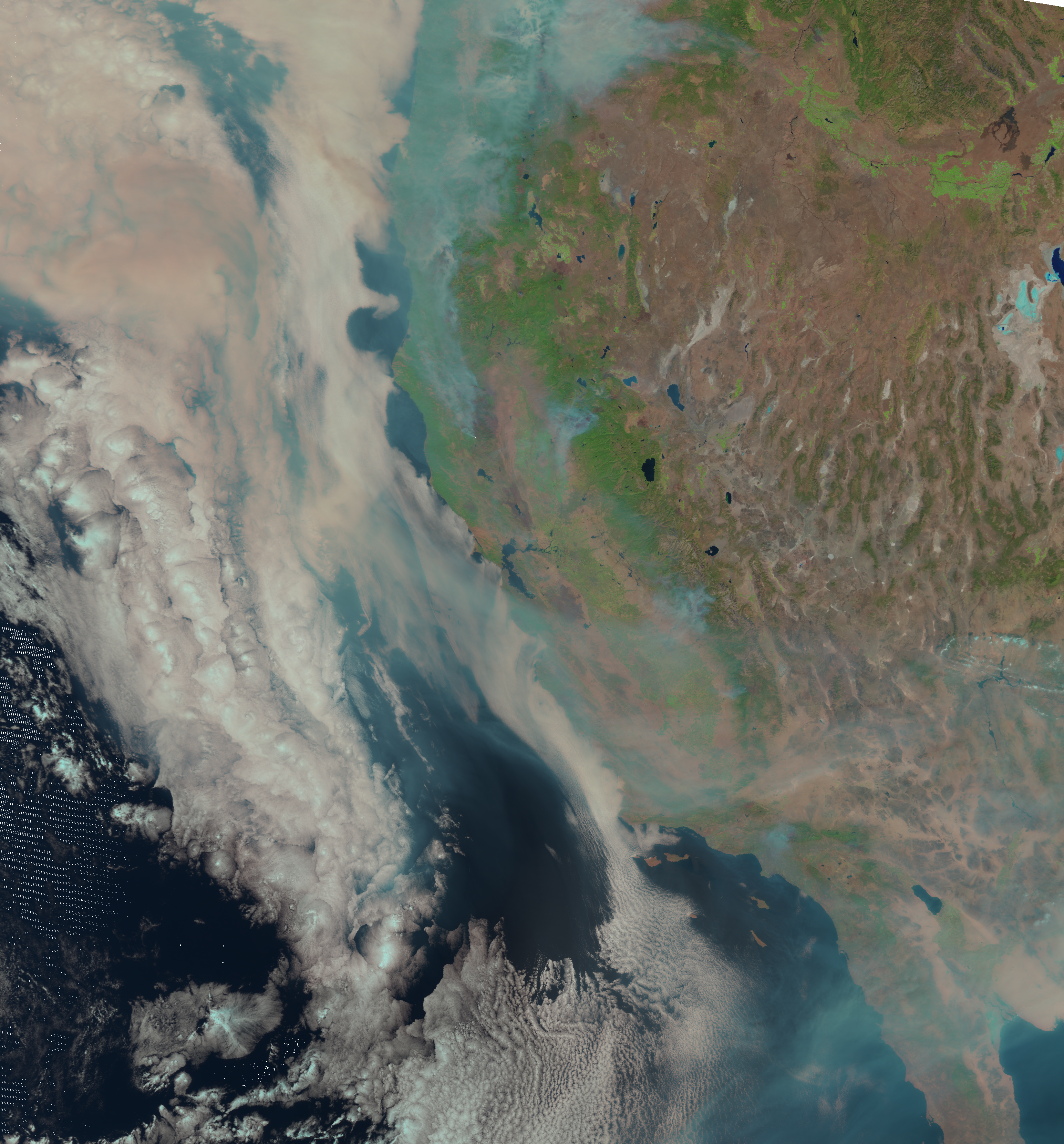
Visualize MODIS natural_color RGB composite with Cartopy features

SatPy’s built-in visualization function is nice, but often you want to make use of additonal features, such as country borders. The library Cartopy offers powerful functions that enable the visualization of geospatial data in different projections and to add additional features to a plot. Below, we will show you how you can visualize the natural_color composite with the two Python packages matplotlib and Cartopy.

As a first step, we have to convert the Scene object into a numpy array. The numpy array additionally needs to be transposed to a shape that can be interpreted by matplotlib’s function imshow(): (M,N,3). You can convert a Scene object into a numpy.array object with the function np.asarray().

The shape of the array is (3, 3320, 3089). This means we have to transpose the array and add index=0 on index position 3.

shape = np.asarray(scn_resample["natural_color"]).shape
shape

(3, 3320, 3089)

Now, we can use .transpose() to transpose the array.

image = np.asarray(scn_resample["natural_color"]).transpose(1,2,0)

The next step is then to replace all nan values with 0. You can do this with the numpy function nan_to_num(). In a subsequent step, we then scale the values to the range between 0 and 1, clipping the lower and upper percentiles so that a potential contrast decrease caused by outliers is eliminated.

image = np.nan_to_num(image)
image = np.interp(image, (np.percentile(image,1), np.percentile(image,99)), (0, 1))

Let us now also define a variable for the coordinate reference system. We take the area attribute from she scn_resample_nc Scene and convert it with the function to_cartopy_crs() into a format Cartopy can read. We will use the crs information for plotting.

crs = scn_resample["natural_color"].attrs["area"].to_cartopy_crs()

Now, we can visualize the natural_color composite. The plotting code can be divided in four main parts:

• Initiate a matplotlib figure: Initiate a matplotlib plot and define the size of the plot

• Specify coastlines and a grid: specify additional features to be added to the plot

• Plotting function: plot the numpy array with the plotting function imshow()

• Set plot title: specify title of the plot

# Initiate a matplotlib figure
fig = plt.figure(figsize=(16, 10))

ax = fig.add_subplot(1, 1, 1, projection=crs)

# Specify coastlines
ax.coastlines(resolution="10m", color="white")

# Specify a grid
gl = ax.gridlines(draw_labels=True, linestyle='--', xlocs=range(-140,-110,5), ylocs=range(20,50,5))
gl.top_labels=False
gl.right_labels=False
gl.xformatter=LONGITUDE_FORMATTER
gl.yformatter=LATITUDE_FORMATTER
gl.xlabel_style={'size':14}
gl.ylabel_style={'size':14}

# Plotting function
ax.imshow(image, transform=crs, extent=crs.bounds, origin="upper")

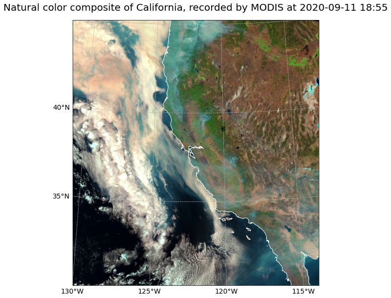
# Set plot title
plt.title("Natural color composite of California, recorded by MODIS at " + scn['1'].attrs['start_time'].strftime("%Y-%m-%d %H:%M"), fontsize=20, pad=20.0)

# Show the plot
plt.show()

---

References

• MODIS Characterization Support Team (MCST), 2017. MODIS 1km Calibrated Radiances Product. NASA MODIS Adaptive Processing System, Goddard Space Flight Center, USA: http://dx.doi.org/10.5067/MODIS/MOD021KM.061

• Some code in this notebook was adapted from the following sources:

  • origin: https://python-kurs.github.io/sommersemester_2019/units/S01E07.html

  • copyright: 2019, Marburg University

  • license: CC BY-SA 4.0

  • retrieved: 2022-06-28 by Sabrina Szeto

Return to the case study

Monitoring smoke transport with next-generation satellites from Metop-SG: Californian Wildfires Case Study
EPS-SG METimage

previous

Monitoring smoke transport with next-generation satellites from Metop-SG

next

Copernicus Sentinel-5P TROPOMI - Ultraviolet Aerosol Index - Level 2