LSA SAF Fire Risk Map v2¶

Hint

Execute the notebook on the training platform >>

The LSA SAF Fire Risk Map v2 (FRMv2) product “combines information from Numerical Weather Prediction (NWP) models - in this case the operational forecasts from ECMWF - and historical SEVIRI estimates of Fire Radiative Power to derive forecasts of the risk of fire. The rationale is to provide the user community with information on meteorological risk that will allow adopting the adequate measures to mitigate fire damage. The FRM algorithm computes the probability of a fires reaching very high intensities for the following 24h, 48h, … 120h. These indicate prognostic levels of fire danger over Southern Europe and part of Northern Africa.” (Source)

This notebook shows the structure of LSA SAF Fire Risk Map v2 (FRMv2) data and what information of the data files can be used in order to load, browse and visualize the data.

The events featured in this notebook are the wildfires in Italy and Greece in summer 2021.

Basic Facts

Spatial resolution: 3km
Spatial coverage: Mediterranean Europe
Time steps: Daily forecasts (24-hr up to 120-hr ahead)
Data availability: since 2017

How to access the data

The FRMv2 data can be accessed via LSA SAF. The data are distributed in HDF5 format, which is then compressed as a TAR file for download.

You need to register for an account before being able to download data.

Load required libraries

import os
import glob
import numpy as np
import datetime
from datetime import datetime
from osgeo import gdal,osr
import pyproj
import tarfile
import bz2

# Python libraries for visualisation
import matplotlib as mpl
from matplotlib import pyplot as plt
import matplotlib.colors as colors
from matplotlib.colors import BoundaryNorm, ListedColormap, TwoSlopeNorm
import cartopy.crs as ccrs
from cartopy.mpl.gridliner import LONGITUDE_FORMATTER, LATITUDE_FORMATTER

from IPython.display import display, clear_output

import warnings
warnings.filterwarnings('ignore')
warnings.simplefilter(action = "ignore", category = RuntimeWarning)

Load helper functions

%run ../functions.ipynb

Fire Risk Map¶

Load and browse the LSA SAF Fire Risk Map v2 data¶

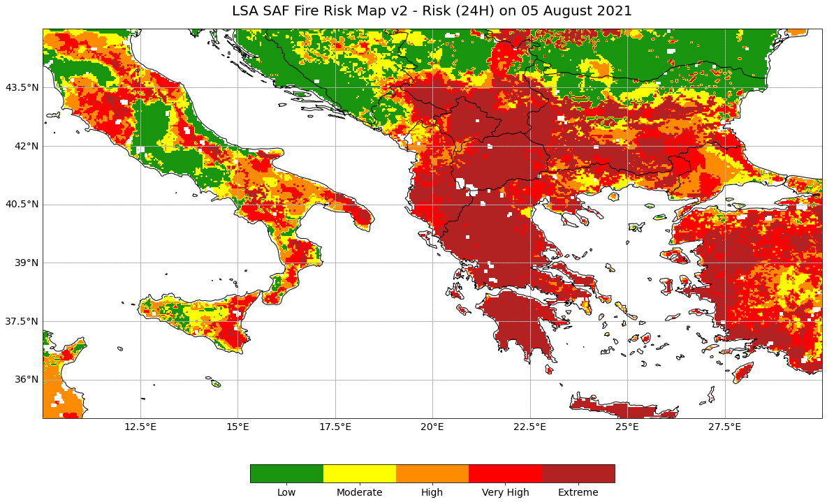
The fire risk map product consists of daily forecasts of classes of meteorological fire danger over Mediterranean Europe. Five fire risk classes are provided, ranging from low to extreme risk. The forecast timesteps available start at 24 hours to 120 hours. The dataset shown here is for the 24 hour forecast.

[OPTIONAL] Unzip the LSA SAF Fire Risk Map v2 data¶

LSA SAF Fire Risk Map v2 data are disseminated in the HDF5 format which is compressed twice, first as a bz2 file individually and then as a group as a TAR file. You can use the library tarfile to open and extract the files. This is optional as we have already unzipped the file for you. This is why the code is commented out.

# Open file
# tar = tarfile.open('../data/lsasaf/frmv2/2021/08/04/order_158116.tar')

# Extract file
# tar.extractall('../data/lsasaf/frmv2/2021/08/04/order_158116')
  
# tar.close()

When you look in the folder containing the extracted files, you will note that the files are compressed individually in bz2 format. You can use bunzip2, which is part of the bzip2 library, to decompress the bz2 files. You use the -k flag to indicate that you want to keep the bz2 archive file and not replace it with the decompressed file. You use the -f flag to indicate that you want to replace any existing files with the same filename.

# %%bash

# bunzip2 -k -f '../data/lsasaf/frmv2/2021/08/04/order_158116/HDF5_LSASAF_MSG_FRM-F024_MSG-Disk_202108051200.bz2'

Inspect structure of LSA SAF Fire Risk Map v2 product data files (24 hour timestep)¶

First, define the filepath for where the hdf5 file(s) are located and store this as the variable in_filepath. You can also define the filepath for where the new tif file(s) will be placed, storing it as the variable out_filepath.

You can also inspect the files in the folder containing the hdf5 files. As we specified a specific file which contains the 24 hour forecast, there should only be a single file in the list.

in_filepath = '../data/lsasaf/frmv2/2021/08/04/order_158116/HDF5_LSASAF_MSG_FRM-F024_MSG-Disk_202108051200'
out_filepath = './outputs'

myfiles = glob.glob(in_filepath)
myfiles

['../data/lsasaf/frmv2/2021/08/04/order_158116/HDF5_LSASAF_MSG_FRM-F024_MSG-Disk_202108051200']

You can use the gdal Python library to access and manipulate datasets in HDF5 format.

[OPTIONAL] Next, you can use the for-loop defined below to process the hdf5 files. We have already done this for you, so the code in the next code block is commented out. There are several steps:

Print file name: The file name is printed out.
Modify file name: The .hdf file ending is split off and a .tif ending is added. A second file is created with the _rep.tif ending; “rep” stands for reprojected.
Translate data:The satellite height and elliptical values are translated to xy values in the new .tif file using the gdal_translate function. At this step we pass in the internal path to the fire risk data which is ://Risk.
Warp data: The values are mapped out and stored in the new _rep.tif file using gdalwarp.

'''
for f in myfiles:
    filename = f.split("\\")[-1]
    print("filename:",filename,"\n")
    
    # Modify file name
    f_out = filename + ".tif"  
    print("f_out:",f_out,"\n")
    
    f_rep = filename + "_rep.tif" 
    print("f_rep:",f_rep,"\n")
    
    # Translate data
    os.system('gdal_translate -of GTiff -a_srs "+proj=geos +h=35785831 +a=6378169 +b=6356583.8 +no_defs"\
    -a_ullr  -5568748.27576  5568748.27576 5568748.27576 -5568748.27576 HDF5:'+ filename +'://Risk '+ f_out)
    
    # Warp data
    os.system('gdalwarp -ot Float32 -s_srs "+proj=geos +h=35785831 +a=6378169 +b=6356583.8 +no_defs"\
    -t_srs EPSG:4326 -r near -of GTiff ' + f_out + ' ' + f_rep)
   
print('done.')
'''

Next, you can enable exceptions in the gdal library to be notified in case of a failure. Then you define the file path to the reprojected tif file and open it using gdal.Open().

gdal.UseExceptions()

rep_file = '../data/lsasaf/frmv2/2021/08/04/order_158116/HDF5_LSASAF_MSG_FRM-F024_MSG-Disk_202108051200_rep.tif' 
ds = gdal.Open(rep_file)

You can take a look at some attributes from the reprojected tif file, such as the number of columns, rows, bands and the driver.

cols = ds.RasterXSize
print('The number of columns is ',cols)
rows = ds.RasterYSize
print('The number of rows is ', rows)
bands = ds.RasterCount
print('The number of bands is ', bands)
driver = ds.GetDriver().LongName
print('The driver is ', driver)

The number of columns is  3879
The number of rows is  3537
The number of bands is  1
The driver is  GeoTIFF

Next, you can access the metadata from the dataset using the gdal function .GetMetadata(). Then, print out the metadata to see what is available.

meta = ds.GetMetadata()
for i in meta: 
    print(i)

ARCHIVE_FACILITY
AREA_OR_POINT
ASSOCIATED_QUALITY_INFORMATION
CENTRE
CFAC
CLOUD_COVERAGE
COFF
COMPRESSION
DISPOSITION_FLAG
END_ORBIT_NUMBER
FIELD_TYPE
FORECAST_STEP
GRANULE_TYPE
IMAGE_ACQUISITION_TIME
INSTRUMENT_ID
INSTRUMENT_MODE
LFAC
LOFF
NB_PARAMETERS
NC
NL
NOMINAL_LAT
NOMINAL_LONG
NOMINAL_PRODUCT_TIME
ORBIT_TYPE
OVERALL_QUALITY_FLAG
PARENT_PRODUCT_NAME
PIXEL_SIZE
PROCESSING_LEVEL
PROCESSING_MODE
PRODUCT
PRODUCT_ACTUAL_SIZE
PRODUCT_ALGORITHM_VERSION
PRODUCT_TYPE
PROJECTION_NAME
REGION_NAME
SAF
SATELLITE
SENSING_END_TIME
SENSING_START_TIME
SPECTRAL_CHANNEL_ID
START_ORBIT_NUMBER
STATISTIC_TYPE
SUB_SATELLITE_POINT_END_LAT
SUB_SATELLITE_POINT_END_LON
SUB_SATELLITE_POINT_START_LAT
SUB_SATELLITE_POINT_START_LON
TIME_RANGE

You can extract the value of a metadata property by using [] square brackets and passing in the name of the property. Let’s extract the 'PRODUCT' metadata value.

product = meta['PRODUCT']
product

'FRM'

You can use these metadata properties in your final plot. For example, you can extract the date from 'IMAGE_ACQUISITION_TIME', turn it into a datetime object and then reformat it for use in your plot.

date = meta['IMAGE_ACQUISITION_TIME']
date

'20210805120000'

timestamp = datetime.strptime(date, '%Y%m%d%H%M%S')
timestamp

datetime.datetime(2021, 8, 5, 12, 0)

title_time = timestamp.strftime('%d %B %Y')
title_time

'05 August 2021'

Visualise the LSA SAF Fire Risk Map v2 data¶

To plot the data, you first need to read in the data as as numpy array, using the function .ReadAsArray(). Then you can mask out the data where the values are equal or less than the missing value of -8000.

data = ds.ReadAsArray()
data = np.ma.masked_where(data <= -8000, data)

You can make use of the ListedColorMap function from the matplotlib library to define the colors for each fire risk class.

cmap = ListedColormap([[24/255., 148/255., 15/255.],
                      [255./255., 255./255., 0],
                      [1., 140./255., 0], [1, 0, 0],
                      [178./255., 34./255., 34./255.]])

You can define the levels for the respective fire risk classes in a list stored in the variable bounds. The fire risk data has a categorical range from 1 to 5, from low to extreme risk. You can also use the .BoundaryNorm() function from matplotlib.colors to define the norm that you will use for plotting later.

bounds = [0,1.5,2.5,3.5,4.5,5.5]
norm = mpl.colors.BoundaryNorm(bounds, cmap.N)  

Finally, you can visualise the fire risk data by plotting it.

The plotting code can be divided in five main parts:

Define the coordinate reference system for the plot
Initiate a matplotlib figure: Initiate a matplotlib plot and define the size of the plot
Specify coastlines, borders and a grid: specify additional features to be added to the plot
Plotting function: specify the extent and plot the data with the plotting function imshow()
Set plot title: specify title of the plot

# Define the coordinate reference system
crs = ccrs.PlateCarree()

# Initiate a matplotlib figure
fig=plt.figure(figsize=(20, 12))
ax = plt.axes(projection=crs)

# Specify coastlines and borders
ax.coastlines(zorder=3)
ax.add_feature(cfeature.BORDERS, edgecolor='black', linewidth=1, zorder=3)

# Specify a grid
gl = ax.gridlines(crs=crs)
gl = ax.gridlines(draw_labels=True, linestyle='--')
gl.top_labels=False
gl.right_labels=False
gl.xformatter=LONGITUDE_FORMATTER
gl.yformatter=LATITUDE_FORMATTER
gl.xlabel_style={'size':14}
gl.ylabel_style={'size':14}

# Set extent of the plot to the Mediterranean 
ax.set_extent([10, 30, 35, 45])

# Define the image extent
img_extent = (-81.26765645410755,81.26765645410755,-74.11423113858775,74.11423113858775)

# Plot the data
cax = ax.imshow(data, cmap=cmap, origin='upper', extent=img_extent, transform=crs, norm=norm)

# Define the colorbar, tick locations and tick labels 
cbar = fig.colorbar(cax, ax=ax, orientation='horizontal', fraction=0.04, pad=0.1, ticks=[0.75,2,3,4,5])
cbar.ax.set_xticklabels(['Low','Moderate','High','Very High','Extreme'])
cbar.ax.tick_params(labelsize=14)

# Set the title of the plot
ax.set_title('LSA SAF Fire Risk Map v2 - Risk (24H) on ' + title_time, fontsize=20, pad=20.0)

# Show the plot
plt.show()

../_images/figure234_LSA_SAF_FRMv2_45_0.png

Return to the case study

Assessing pre-fire risk with next-generation satellites: Mediterranean Fires Case Study
Fire Risk Map: fire risk, fire probability and fire probability anomalies

P2000¶

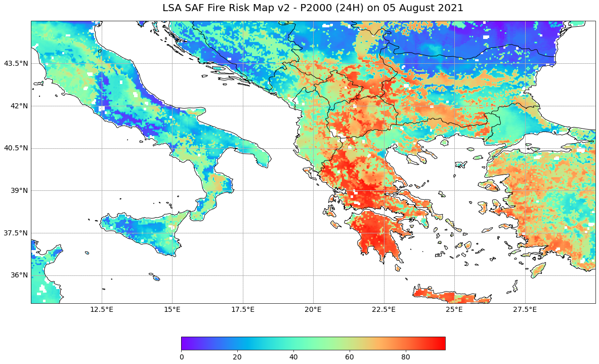
Probabilities of a Potential Wildfire exceeding 2000 GJ of Daily Energy released by Fires¶

The P2000 dataset shows the probabilities of a potential wildfire exceeding 2000 GJ of daily energy released by fires. In other words, it provides information on the likelihood of a potential wildfire getting out of control.

Load and browse the LSA SAF P2000 data¶

You can reuse the variables in_filepath and out_filepath that you defined earlier.

You can use the gdal Python library to access and manipulate datasets in HDF5 format.

[OPTIONAL] Next, you can use the for-loop defined below to process the hdf5 files. We have already done this for you, so the code in the next code block is commented out. There are several steps:

Print file name: The file name is printed out.
Modify file name: The .hdf file ending is split off and a .tif ending is added. A second file is created with the _rep.tif ending; “rep” stands for reprojected.
Translate data:The satellite height and elliptical values are translated to xy values in the new .tif file using the gdal_translate function. At this step we pass in the internal path to the P2000 data which is P2000.
Warp data: The values are mapped out and stored in the new _rep.tif file using gdalwarp.

'''
for f in myfiles:
    
    # Print file name
    filename = f.split("\\")[-1]
    print("filename:",filename,"\n")
    
    # Modify file name
    f_out = filename +"_p2000" + ".tif"  
    print("f_out:",f_out,"\n")
    
    f_rep = filename +"_p2000" + "_rep.tif" 
    print("f_rep:",f_rep,"\n")
    
    # Translate data
    os.system('gdal_translate -of GTiff -a_srs "+proj=geos +h=35785831 +a=6378169 +b=6356583.8 +no_defs"\
    -a_ullr  -5568748.27576  5568748.27576 5568748.27576 -5568748.27576 HDF5:'+ filename +'://P2000 '+ f_out)
    
    # Warp data
    os.system('gdalwarp -ot Float32 -s_srs "+proj=geos +h=35785831 +a=6378169 +b=6356583.8 +no_defs"\
    -t_srs EPSG:4326 -r near -of GTiff ' + f_out + ' ' + f_rep)
   
print('done.')
'''

Next, define the file path to the reprojected tif file and open it using gdal.Open().

p2000_file = '../data/lsasaf/frmv2/2021/08/04/order_158116/HDF5_LSASAF_MSG_FRM-F024_MSG-Disk_202108051200_p2000_rep.tif'
p2000_ds = gdal.Open(p2000_file)

Visualise the LSA SAF P2000 data¶

To plot the data, you first need to read in the data as as numpy array, using the function .ReadAsArray(). Then you can mask out the data where the values are equal or less than the missing value of -8000.

p2000_data = p2000_ds.ReadAsArray()
p2000_data = np.ma.masked_where(p2000_data <= -8000, p2000_data)

Finally, you can visualise the fire risk data by plotting it.

The plotting code can be divided in five main parts:

Define the coordinate reference system for the plot
Initiate a matplotlib figure: Initiate a matplotlib plot and define the size of the plot
Specify coastlines, borders and a grid: specify additional features to be added to the plot
Plotting function: specify the extent and plot the data with the plotting function imshow()
Set plot title: specify title of the plot

# Define the coordinate reference system
crs = ccrs.PlateCarree()

# Initiate a matplotlib figure
fig = plt.figure(figsize=(20, 12))
ax = plt.axes(projection=crs)

# Specify coastlines and borders
ax.coastlines(zorder=3)
ax.add_feature(cfeature.BORDERS, edgecolor='black', linewidth=1, zorder=3)

# Specify a grid
gl = ax.gridlines(crs=crs)
gl = ax.gridlines(draw_labels=True, linestyle='--')
gl.top_labels=False
gl.right_labels=False
gl.xformatter=LONGITUDE_FORMATTER
gl.yformatter=LATITUDE_FORMATTER
gl.xlabel_style={'size':14}
gl.ylabel_style={'size':14}

# Set extent of the plot to the Mediterranean 
ax.set_extent([10, 30, 35, 45])

# Define the image extent (the extent of the data)
img_extent = (-81.26765645410755,81.26765645410755,-74.11423113858775,74.11423113858775)

# Plot the data
cax = ax.imshow(p2000_data, cmap="rainbow", origin='upper', extent=img_extent, transform=crs)

# Define the colorbar
cbar = fig.colorbar(cax, ax=ax, orientation='horizontal', fraction=0.04, pad=0.1)
cbar.ax.tick_params(labelsize=14)

# Set the title of the plot
ax.set_title('LSA SAF Fire Risk Map v2 - P2000 (24H) on ' + title_time, fontsize=20, pad=20.0)

# Show the plot
plt.show()

../_images/figure234_LSA_SAF_FRMv2_61_0.png

Return to the case study

Assessing pre-fire risk with next-generation satellites: Mediterranean Fires Case Study
Probabilities of a Potential Wildfire exceeding 2000 GJ of Daily Energy released by Fires (P2000)

P2000a¶

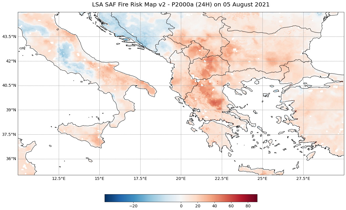
24 hour forecast of the anomaly of probability of exceedance of 2000 GJ of daily energy released by fires (P2000a)¶

This anomaly is computed at each pixel as the deviation of the probability of exceedance for a given pixel and a given day of a given year from the average of all values of probability of exceedance for that pixel and day over the period 1979–2016.

Load and browse the LSA SAF P2000a data¶

You can reuse the variables in_filepath and out_filepath that you defined earlier.

You can use the gdal Python library to access and manipulate datasets in HDF5 format.

[OPTIONAL] Next, you can use the for-loop defined below to process the hdf5 files. We have already done this for you, so the code in the next code block is commented out. There are several steps:

Print file name: The file name is printed out.
Modify file name: The .hdf file ending is split off and a .tif ending is added. A second file is created with the _rep.tif ending; “rep” stands for reprojected.
Translate data:The satellite height and elliptical values are translated to xy values in the new .tif file using the gdal_translate function. At this step we pass in the internal path to the P2000a data which is P2000a.
Warp data: The values are mapped out and stored in the new _rep.tif file using gdalwarp.

'''
for f in myfiles:
    
    # Print file name
    filename = f.split("\\")[-1]
    print("filename:",filename,"\n")
    
    # Modify file name
    f_out = filename +"_p2000a" + ".tif"
    print("f_out:",f_out,"\n")
    
    f_rep = filename +"_p2000a" + "_rep.tif" 
    print("f_rep:",f_rep,"\n")
    
    # Translate data
    os.system('gdal_translate -of GTiff -a_srs "+proj=geos +h=35785831 +a=6378169 +b=6356583.8 +no_defs"\
    -a_ullr  -5568748.27576  5568748.27576 5568748.27576 -5568748.27576 HDF5:'+ filename +'://P2000a '+ f_out)
    
    # Warp data
    os.system('gdalwarp -ot Float32 -s_srs "+proj=geos +h=35785831 +a=6378169 +b=6356583.8 +no_defs"\
    -t_srs EPSG:4326 -r near -of GTiff ' + f_out + ' ' + f_rep)
   
print('done.')
'''

Next, define the file path to the reprojected tif file and open it using gdal.Open().

p2000a_file = '../data/lsasaf/frmv2/2021/08/04/order_158116/HDF5_LSASAF_MSG_FRM-F024_MSG-Disk_202108051200_p2000a_rep.tif'
p2000a_ds = gdal.Open(p2000a_file)

Visualise the LSA SAF P2000a data¶

To plot the data, you first need to read in the data as as numpy array, using the function .ReadAsArray(). Then you can mask out the data where the values are equal or less than the missing value of -8000.

p2000a_data = p2000a_ds.ReadAsArray()
p2000a_data = np.ma.masked_where(p2000a_data <= -8000, p2000a_data)

Finally, you can visualise the fire risk data by plotting it.

The plotting code can be divided in five main parts:

Define the coordinate reference system for the plot
Initiate a matplotlib figure: Initiate a matplotlib plot and define the size of the plot
Specify coastlines, borders and a grid: specify additional features to be added to the plot
Plotting function: specify the extent and plot the data with the plotting function imshow()
Set plot title: specify title of the plot

# Define the coordinate reference system
crs = ccrs.PlateCarree()

# Initiate a matplotlib figure
fig = plt.figure(figsize=(20, 12))
ax = plt.axes(projection=crs)

# Specify coastlines and borders
ax.coastlines(zorder=3)
ax.add_feature(cfeature.BORDERS, edgecolor='black', linewidth=1, zorder=3)

# Specify a grid
gl = ax.gridlines(crs=crs)
gl = ax.gridlines(draw_labels=True, linestyle='--')
gl.top_labels=False
gl.right_labels=False
gl.xformatter=LONGITUDE_FORMATTER
gl.yformatter=LATITUDE_FORMATTER
gl.xlabel_style={'size':14}
gl.ylabel_style={'size':14}

# Set extent of the plot to the Mediterranean 
ax.set_extent([10, 30, 35, 45]) # Mediterranean

# Define the image extent (the extent of the data)
img_extent = (-81.26765645410755,81.26765645410755,-74.11423113858775,74.11423113858775)

# Center white part of color ramp on 0
norm = TwoSlopeNorm(vmin=p2000a_data.min(), vcenter=0, vmax=p2000a_data.max())

# Plot the data
cax = ax.imshow(p2000a_data, cmap="RdBu_r", norm=norm, origin='upper', extent=img_extent, transform=crs)

# Define the colorbar
cbar = fig.colorbar(cax, ax=ax, orientation='horizontal', fraction=0.04, pad=0.1)
cbar.ax.tick_params(labelsize=14)

# Set the title of the plot
ax.set_title('LSA SAF Fire Risk Map v2 - P2000a (24H) on ' + title_time, fontsize=20, pad=20.0)

# Show the plot
plt.show()

../_images/figure234_LSA_SAF_FRMv2_77_0.png

References¶

Trigo, I. F., C. C. DaCamara, P. Viterbo, J.-L. Roujean, F. Olesen, C. Barroso, F. Camacho-de Coca, D. Carrer, S. C. Freitas, J. García-Haro, B. Geiger, F. Gellens-Meulenberghs, N. Ghilain, J. Meliá, L. Pessanha, N. Siljamo, and A. Arboleda. (2011). The Satellite Application Facility on Land Surface Analysis. Int. J. Remote Sens., 32, 2725-2744, doi: 10.1080/01431161003743199
Some code in this notebook was adapted from the following source:
- origin: https://stackoverflow.com/questions/53643062/lsa-saf-satellite-hdf5-plot-in-python-cartopy
- copyright: 2018, methane rain
- license: CC BY-SA 4.0
- retrieved: 2022-06-28 by Sabrina Szeto

Return to the case study

Assessing pre-fire risk with next-generation satellites: Mediterranean Fires Case Study
24 hour forecast of the anomaly of probability of exceedance of 2000 GJ of daily energy released by fires (P2000a)

FANGS - Fire Applications with Next-Generation Satellites

LSA SAF Fire Risk Map v2

Contents

LSA SAF Fire Risk Map v2¶

Fire Risk Map¶

Load and browse the LSA SAF Fire Risk Map v2 data¶

[OPTIONAL] Unzip the LSA SAF Fire Risk Map v2 data¶

Inspect structure of LSA SAF Fire Risk Map v2 product data files (24 hour timestep)¶

Visualise the LSA SAF Fire Risk Map v2 data¶

P2000¶

Probabilities of a Potential Wildfire exceeding 2000 GJ of Daily Energy released by Fires¶

Load and browse the LSA SAF P2000 data¶

Visualise the LSA SAF P2000 data¶

P2000a¶

24 hour forecast of the anomaly of probability of exceedance of 2000 GJ of daily energy released by fires (P2000a)¶

Load and browse the LSA SAF P2000a data¶

Visualise the LSA SAF P2000a data¶

References¶