Copernicus Sentinel-5P TROPOMI - Ultraviolet Aerosol Index - Level 2
Contents
Copernicus Sentinel-5P TROPOMI - Ultraviolet Aerosol Index - Level 2
The Copernicus Sentinel-5 Ultraviolet Visible Near-Infrared Shortwave (UVNS) spectrometer enables the measurement of trace gases which will improve air quality forecasts produced by the Copernicus Atmosphere Monitoring service.
This notebook provides you an introduction to data from Sentinel-5P, the precursor instrument and proxy for data from Sentinel-5. Sentinel-5P data can be downloaded from the Sentinel-5P Pre-Operations Data Hub.
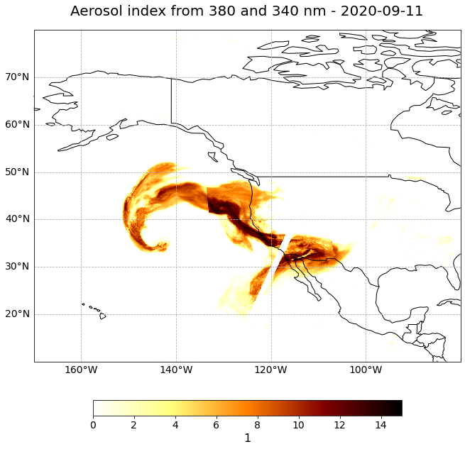
The event featured is the August Complex fire in California, USA in 2020. This was the largest wildfire in CA history, spreading over 1,000,000 acres (over 4,000 sq km). The image shown in this notebook is taken from 11 September 2020.
For monitoring smoke, the TROPOMI UV Aerosol Index (UVAI) data can be used. Positive values of UVAI (typically > about 1.0) indicate the presence of absorbing-type aerosols:
smoke from forest fires,volcanic ash, ordesert dust.
Basic Facts
Spatial resolution: Up to 5.5* km x 3.5 km (5.5 km in the satellite flight direction and 3.5 km in the perpendicular direction at nadir)
Spatial coverage: Global
Revisit time: less than one day
Data availability: since April 2018
How to access the data
Sentinel-5P Pre-Ops data are disseminated in the netCDF format and can be downloaded via the Copernicus Open Access Hub. You need to register for an account before downloading data.
Load required libraries
import os
import xarray as xr
from datetime import datetime
import numpy as np
from netCDF4 import Dataset
import pandas as pd

# Python libraries for visualization
import matplotlib.pyplot as plt
import matplotlib.colors
import matplotlib.cm as cm
from matplotlib.axes import Axes
import cartopy
import cartopy.crs as ccrs
from cartopy.mpl.gridliner import LONGITUDE_FORMATTER, LATITUDE_FORMATTER
from cartopy.mpl.geoaxes import GeoAxes
GeoAxes._pcolormesh_patched = Axes.pcolormesh
from skimage import exposure

import warnings
warnings.filterwarnings('ignore')
warnings.simplefilter(action = "ignore", category = RuntimeWarning)
Load helper functions
%run ../functions.ipynb
Load and browse Sentinel-5P TROPOMI Aerosol Index Level 2 data
A Sentinel-5P TROPOMI Aerosol Index Level 2 file is organised in two groups: PRODUCT and METADATA. The PRODUCT group stores the main data fields of the product, including latitude, longitude and the variable itself. The METADATA group provides additional metadata items.
Sentinel-5P TROPOMI variables have the following dimensions:
scanline: the number of measurements in the granule / along-track dimension indexground_pixel: the number of spectra in a measurement / across-track dimension indextime: time reference for the datacorner: pixel corner index
Sentinel-5P TROPOMI data is disseminated in netCDF. You can load several netCDF files with the open_mfdataset() function of the xarray library. In order to load the variable as part of a Sentinel-5P data files, you have to specify the following keyword arguments:
concat_dim='scanline': to concatenate the dimensions along the scanlinecombine='nested': to combine the data of an n-dimensionsional array into one by using a succession of concatenate and merge operations along each dimension of the grid.group='PRODUCT': to load thePRODUCTgroup
You can load all the datasets available for one day into one xarray object by using scanline as concatanation dimension.
s5p_mf = xr.open_mfdataset('../data/sentinel-5p/uvai/2020/09/11/*.nc', concat_dim='scanline', combine='nested', group='PRODUCT')
s5p_mf
<xarray.Dataset>
Dimensions:                          (scanline: 12079, ground_pixel: 450, time: 1, corner: 4)
Coordinates:
  * scanline                         (scanline) float64 0.0 1.0 ... 3.734e+03
  * ground_pixel                     (ground_pixel) float64 0.0 1.0 ... 449.0
  * time                             (time) datetime64[ns] 2020-09-11
  * corner                           (corner) float64 0.0 1.0 2.0 3.0
    latitude                         (time, scanline, ground_pixel) float32 dask.array<chunksize=(1, 4172, 450), meta=np.ndarray>
    longitude                        (time, scanline, ground_pixel) float32 dask.array<chunksize=(1, 4172, 450), meta=np.ndarray>
Data variables:
    delta_time                       (time, scanline) datetime64[ns] dask.array<chunksize=(1, 4172), meta=np.ndarray>
    time_utc                         (time, scanline) object dask.array<chunksize=(1, 4172), meta=np.ndarray>
    qa_value                         (time, scanline, ground_pixel) float32 dask.array<chunksize=(1, 4172, 450), meta=np.ndarray>
    aerosol_index_354_388            (time, scanline, ground_pixel) float32 dask.array<chunksize=(1, 4172, 450), meta=np.ndarray>
    aerosol_index_340_380            (time, scanline, ground_pixel) float32 dask.array<chunksize=(1, 4172, 450), meta=np.ndarray>
    aerosol_index_354_388_precision  (time, scanline, ground_pixel) float32 dask.array<chunksize=(1, 4172, 450), meta=np.ndarray>
aerosol_index_340_380_precision (time, scanline, ground_pixel) float32 dask.array<chunksize=(1, 4172, 450), meta=np.ndarray>- scanline: 12079
- ground_pixel: 450
- time: 1
- corner: 4
- scanline(scanline)float640.0 1.0 2.0 ... 3.733e+03 3.734e+03
- units :
- 1
- axis :
- Y
- long_name :
- along-track dimension index
- comment :
- This coordinate variable defines the indices along track; index starts at 0
array([0.000e+00, 1.000e+00, 2.000e+00, ..., 3.732e+03, 3.733e+03, 3.734e+03])
- ground_pixel(ground_pixel)float640.0 1.0 2.0 ... 447.0 448.0 449.0
- units :
- 1
- axis :
- X
- long_name :
- across-track dimension index
- comment :
- This coordinate variable defines the indices across track, from west to east; index starts at 0
array([ 0., 1., 2., ..., 447., 448., 449.])
- time(time)datetime64[ns]2020-09-11
- standard_name :
- time
- axis :
- T
- long_name :
- reference time for the measurements
- comment :
- The time in this variable corresponds to the time in the time_reference global attribute
array(['2020-09-11T00:00:00.000000000'], dtype='datetime64[ns]')
- corner(corner)float640.0 1.0 2.0 3.0
- units :
- 1
- long_name :
- pixel corner index
- comment :
- This coordinate variable defines the indices for the pixel corners; index starts at 0 (counter-clockwise, starting from south-western corner of the pixel in ascending part of the orbit)
array([0., 1., 2., 3.])
- latitude(time, scanline, ground_pixel)float32dask.array<chunksize=(1, 4172, 450), meta=np.ndarray>
- long_name :
- pixel center latitude
- units :
- degrees_north
- standard_name :
- latitude
- valid_min :
- -90.0
- valid_max :
- 90.0
- bounds :
- /PRODUCT/SUPPORT_DATA/GEOLOCATIONS/latitude_bounds
Array Chunk Bytes 20.73 MiB 7.16 MiB Shape (1, 12079, 450) (1, 4172, 450) Count 9 Tasks 3 Chunks Type float32 numpy.ndarray - longitude(time, scanline, ground_pixel)float32dask.array<chunksize=(1, 4172, 450), meta=np.ndarray>
- long_name :
- pixel center longitude
- units :
- degrees_east
- standard_name :
- longitude
- valid_min :
- -180.0
- valid_max :
- 180.0
- bounds :
- /PRODUCT/SUPPORT_DATA/GEOLOCATIONS/longitude_bounds
Array Chunk Bytes 20.73 MiB 7.16 MiB Shape (1, 12079, 450) (1, 4172, 450) Count 9 Tasks 3 Chunks Type float32 numpy.ndarray
- delta_time(time, scanline)datetime64[ns]dask.array<chunksize=(1, 4172), meta=np.ndarray>
- long_name :
- offset of start time of measurement relative to time_reference
Array Chunk Bytes 94.37 kiB 32.59 kiB Shape (1, 12079) (1, 4172) Count 9 Tasks 3 Chunks Type datetime64[ns] numpy.ndarray - time_utc(time, scanline)objectdask.array<chunksize=(1, 4172), meta=np.ndarray>
- long_name :
- Time of observation as ISO 8601 date-time string
Array Chunk Bytes 94.37 kiB 32.59 kiB Shape (1, 12079) (1, 4172) Count 9 Tasks 3 Chunks Type object numpy.ndarray - qa_value(time, scanline, ground_pixel)float32dask.array<chunksize=(1, 4172, 450), meta=np.ndarray>
- units :
- 1
- valid_min_ :
- 0
- valid_max_ :
- 100
- long_name :
- data quality value
- comment :
- A continuous quality descriptor, varying between 0 (no data) and 1 (full quality data). Recommend to ignore data with qa_value < 0.5
Array Chunk Bytes 20.73 MiB 7.16 MiB Shape (1, 12079, 450) (1, 4172, 450) Count 9 Tasks 3 Chunks Type float32 numpy.ndarray - aerosol_index_354_388(time, scanline, ground_pixel)float32dask.array<chunksize=(1, 4172, 450), meta=np.ndarray>
- units :
- 1
- proposed_standard_name :
- ultraviolet_aerosol_index
- comment :
- Aerosol index from 388 and 354 nm
- long_name :
- Aerosol index from 388 and 354 nm
- radiation_wavelength :
- [354. 388.]
- ancillary_variables :
- aerosol_index_354_388_precision
Array Chunk Bytes 20.73 MiB 7.16 MiB Shape (1, 12079, 450) (1, 4172, 450) Count 9 Tasks 3 Chunks Type float32 numpy.ndarray - aerosol_index_340_380(time, scanline, ground_pixel)float32dask.array<chunksize=(1, 4172, 450), meta=np.ndarray>
- units :
- 1
- proposed_standard_name :
- ultraviolet_aerosol_index
- comment :
- Aerosol index from 380 and 340 nm
- long_name :
- Aerosol index from 380 and 340 nm
- radiation_wavelength :
- [340. 380.]
- ancillary_variables :
- aerosol_index_340_380_precision
Array Chunk Bytes 20.73 MiB 7.16 MiB Shape (1, 12079, 450) (1, 4172, 450) Count 9 Tasks 3 Chunks Type float32 numpy.ndarray - aerosol_index_354_388_precision(time, scanline, ground_pixel)float32dask.array<chunksize=(1, 4172, 450), meta=np.ndarray>
- units :
- 1
- proposed_standard_name :
- ultraviolet_aerosol_index standard_error
- comment :
- Precision of aerosol index from 388 and 354 nm
- long_name :
- Precision of aerosol index from 388 and 354 nm
- radiation_wavelength :
- [354. 388.]
Array Chunk Bytes 20.73 MiB 7.16 MiB Shape (1, 12079, 450) (1, 4172, 450) Count 9 Tasks 3 Chunks Type float32 numpy.ndarray - aerosol_index_340_380_precision(time, scanline, ground_pixel)float32dask.array<chunksize=(1, 4172, 450), meta=np.ndarray>
- units :
- 1
- proposed_standard_name :
- ultraviolet_aerosol_index standard_error
- comment :
- Precision of aerosol index from 380 and 340 nm
- long_name :
- Precision of aerosol index from 380 and 340 nm
- radiation_wavelength :
- [340. 380.]
Array Chunk Bytes 20.73 MiB 7.16 MiB Shape (1, 12079, 450) (1, 4172, 450) Count 9 Tasks 3 Chunks Type float32 numpy.ndarray
You see that the loaded data object contains of four dimensions and seven data variables:
Dimensions:
scanlineground_pixeltimecorner
Data variables:
delta_time: the offset of individual measurements within the granule, given in millisecondstime_utc: valid time stamp of the dataqa_value: quality descriptor, varying between 0 (nodata) and 1 (full quality data).aerosol_index_354_388: Aerosol index from 354 and 388 nmaerosol_index_340_380: Aerosol index from 340 and 380 nmaerosol_index_354_388_precision: Precision of aerosol index from 354 and 388 nmaerosol_index_340_380_precision: Precision of aerosol index from 340 and 380 nm
Retrieve the variable ‘Aerosol index from 340 and 380 nm’ as xarray.DataArray
You can specify one variable of interest by putting the name of the variable into square brackets [] and get more detailed information about the variable. E.g. aerosol_index_340_380 is the ‘Aerosol index from 340 and 380 nm’ and has three dimensions, time, scanline and ground_pixel respectively.
uvai = s5p_mf.aerosol_index_340_380[0,:,:]
uvai
<xarray.DataArray 'aerosol_index_340_380' (scanline: 12079, ground_pixel: 450)>
dask.array<getitem, shape=(12079, 450), dtype=float32, chunksize=(4172, 450), chunktype=numpy.ndarray>
Coordinates:
  * scanline      (scanline) float64 0.0 1.0 2.0 ... 3.733e+03 3.734e+03
  * ground_pixel  (ground_pixel) float64 0.0 1.0 2.0 3.0 ... 447.0 448.0 449.0
    time          datetime64[ns] 2020-09-11
    latitude      (scanline, ground_pixel) float32 dask.array<chunksize=(4172, 450), meta=np.ndarray>
    longitude     (scanline, ground_pixel) float32 dask.array<chunksize=(4172, 450), meta=np.ndarray>
Attributes:
    units:                   1
    proposed_standard_name:  ultraviolet_aerosol_index
    comment:                 Aerosol index from 380 and 340 nm
    long_name:               Aerosol index from 380 and 340 nm
    radiation_wavelength:    [340. 380.]
ancillary_variables: aerosol_index_340_380_precision- scanline: 12079
- ground_pixel: 450
- dask.array<chunksize=(4172, 450), meta=np.ndarray>
Array Chunk Bytes 20.73 MiB 7.16 MiB Shape (12079, 450) (4172, 450) Count 12 Tasks 3 Chunks Type float32 numpy.ndarray - scanline(scanline)float640.0 1.0 2.0 ... 3.733e+03 3.734e+03
- units :
- 1
- axis :
- Y
- long_name :
- along-track dimension index
- comment :
- This coordinate variable defines the indices along track; index starts at 0
array([0.000e+00, 1.000e+00, 2.000e+00, ..., 3.732e+03, 3.733e+03, 3.734e+03])
- ground_pixel(ground_pixel)float640.0 1.0 2.0 ... 447.0 448.0 449.0
- units :
- 1
- axis :
- X
- long_name :
- across-track dimension index
- comment :
- This coordinate variable defines the indices across track, from west to east; index starts at 0
array([ 0., 1., 2., ..., 447., 448., 449.])
- time()datetime64[ns]2020-09-11
- standard_name :
- time
- axis :
- T
- long_name :
- reference time for the measurements
- comment :
- The time in this variable corresponds to the time in the time_reference global attribute
array('2020-09-11T00:00:00.000000000', dtype='datetime64[ns]') - latitude(scanline, ground_pixel)float32dask.array<chunksize=(4172, 450), meta=np.ndarray>
- long_name :
- pixel center latitude
- units :
- degrees_north
- standard_name :
- latitude
- valid_min :
- -90.0
- valid_max :
- 90.0
- bounds :
- /PRODUCT/SUPPORT_DATA/GEOLOCATIONS/latitude_bounds
Array Chunk Bytes 20.73 MiB 7.16 MiB Shape (12079, 450) (4172, 450) Count 12 Tasks 3 Chunks Type float32 numpy.ndarray - longitude(scanline, ground_pixel)float32dask.array<chunksize=(4172, 450), meta=np.ndarray>
- long_name :
- pixel center longitude
- units :
- degrees_east
- standard_name :
- longitude
- valid_min :
- -180.0
- valid_max :
- 180.0
- bounds :
- /PRODUCT/SUPPORT_DATA/GEOLOCATIONS/longitude_bounds
Array Chunk Bytes 20.73 MiB 7.16 MiB Shape (12079, 450) (4172, 450) Count 12 Tasks 3 Chunks Type float32 numpy.ndarray
- units :
- 1
- proposed_standard_name :
- ultraviolet_aerosol_index
- comment :
- Aerosol index from 380 and 340 nm
- long_name :
- Aerosol index from 380 and 340 nm
- radiation_wavelength :
- [340. 380.]
- ancillary_variables :
- aerosol_index_340_380_precision
Create a geographical subset for California, USA
You can zoom into a region by specifying a bounding box of interest. Let us set the extent to California with the following bounding box information:
latmin=10.
latmax=80.
lonmin=-170.
lonmax=-80.
Now, let us apply the function generate_geographical_subset to subset the uvai xarray.DataArray. Let us call the new xarray.DataArray uvai.
uvai_subset = generate_geographical_subset(xarray=uvai,
                                             latmin=latmin,
                                             latmax=latmax,
                                             lonmin=lonmin,
                                             lonmax=lonmax)
uvai_subset
<xarray.DataArray 'aerosol_index_340_380' (scanline: 4550, ground_pixel: 450)>
dask.array<where, shape=(4550, 450), dtype=float32, chunksize=(1582, 450), chunktype=numpy.ndarray>
Coordinates:
  * scanline      (scanline) float64 2.101e+03 2.102e+03 ... 3.559e+03 3.56e+03
  * ground_pixel  (ground_pixel) float64 0.0 1.0 2.0 3.0 ... 447.0 448.0 449.0
    time          datetime64[ns] 2020-09-11
    latitude      (scanline, ground_pixel) float32 dask.array<chunksize=(1582, 450), meta=np.ndarray>
    longitude     (scanline, ground_pixel) float32 dask.array<chunksize=(1582, 450), meta=np.ndarray>
Attributes:
    units:                   1
    proposed_standard_name:  ultraviolet_aerosol_index
    comment:                 Aerosol index from 380 and 340 nm
    long_name:               Aerosol index from 380 and 340 nm
    radiation_wavelength:    [340. 380.]
ancillary_variables: aerosol_index_340_380_precision- scanline: 4550
- ground_pixel: 450
- dask.array<chunksize=(1582, 450), meta=np.ndarray>
Array Chunk Bytes 7.81 MiB 2.72 MiB Shape (4550, 450) (1582, 450) Count 66 Tasks 3 Chunks Type float32 numpy.ndarray - scanline(scanline)float642.101e+03 2.102e+03 ... 3.56e+03
- units :
- 1
- axis :
- Y
- long_name :
- along-track dimension index
- comment :
- This coordinate variable defines the indices along track; index starts at 0
array([2101., 2102., 2103., ..., 3558., 3559., 3560.])
- ground_pixel(ground_pixel)float640.0 1.0 2.0 ... 447.0 448.0 449.0
- units :
- 1
- axis :
- X
- long_name :
- across-track dimension index
- comment :
- This coordinate variable defines the indices across track, from west to east; index starts at 0
array([ 0., 1., 2., ..., 447., 448., 449.])
- time()datetime64[ns]2020-09-11
- standard_name :
- time
- axis :
- T
- long_name :
- reference time for the measurements
- comment :
- The time in this variable corresponds to the time in the time_reference global attribute
array('2020-09-11T00:00:00.000000000', dtype='datetime64[ns]') - latitude(scanline, ground_pixel)float32dask.array<chunksize=(1582, 450), meta=np.ndarray>
- long_name :
- pixel center latitude
- units :
- degrees_north
- standard_name :
- latitude
- valid_min :
- -90.0
- valid_max :
- 90.0
- bounds :
- /PRODUCT/SUPPORT_DATA/GEOLOCATIONS/latitude_bounds
Array Chunk Bytes 7.81 MiB 2.72 MiB Shape (4550, 450) (1582, 450) Count 15 Tasks 3 Chunks Type float32 numpy.ndarray - longitude(scanline, ground_pixel)float32dask.array<chunksize=(1582, 450), meta=np.ndarray>
- long_name :
- pixel center longitude
- units :
- degrees_east
- standard_name :
- longitude
- valid_min :
- -180.0
- valid_max :
- 180.0
- bounds :
- /PRODUCT/SUPPORT_DATA/GEOLOCATIONS/longitude_bounds
Array Chunk Bytes 7.81 MiB 2.72 MiB Shape (4550, 450) (1582, 450) Count 15 Tasks 3 Chunks Type float32 numpy.ndarray
- units :
- 1
- proposed_standard_name :
- ultraviolet_aerosol_index
- comment :
- Aerosol index from 380 and 340 nm
- long_name :
- Aerosol index from 380 and 340 nm
- radiation_wavelength :
- [340. 380.]
- ancillary_variables :
- aerosol_index_340_380_precision
You can extract the latitude and longitude information from the subsetted data and save them into new variables for plotting later.
lat = uvai_subset.latitude
lon = uvai_subset.longitude
Visualize Sentinel-5P TROPOMI ‘Aerosol Index from 340 and 350 nm’
The next step is to visualize the dataset. You can use the function visualize_pcolormesh, which makes use of matploblib’s function pcolormesh and the Cartopy library.
With ?visualize_pcolormesh you can open the function’s docstring to see what keyword arguments are needed to prepare your plot.
?visualize_pcolormesh
Signature:
visualize_pcolormesh(
    data_array,
    longitude,
    latitude,
    projection,
    color_scale,
    unit,
    long_name,
    vmin,
    vmax,
    set_global=True,
    lonmin=-180,
    lonmax=180,
    latmin=-90,
    latmax=90,
)
Docstring:
Visualizes a xarray.DataArray with matplotlib's pcolormesh function.

Parameters:
    data_array(xarray.DataArray): xarray.DataArray holding the data values
    longitude(xarray.DataArray): xarray.DataArray holding the longitude values
    latitude(xarray.DataArray): xarray.DataArray holding the latitude values
    projection(str): a projection provided by the cartopy library, e.g. ccrs.PlateCarree()
    color_scale(str): string taken from matplotlib's color ramp reference
    unit(str): the unit of the parameter, taken from the NetCDF file if possible
    long_name(str): long name of the parameter, taken from the NetCDF file if possible
    vmin(int): minimum number on visualisation legend
    vmax(int): maximum number on visualisation legend
    set_global(boolean): optional kwarg, default is True
    lonmin,lonmax,latmin,latmax(float): optional kwarg, set geographic extent is set_global kwarg is set to
                                        False
File:      /tmp/ipykernel_51/1857473499.py
Type:      function
visualize_pcolormesh(data_array=uvai_subset,
                     longitude=lon,
                     latitude=lat,
                     projection=ccrs.PlateCarree(),
                     color_scale='afmhot_r',
                     unit=uvai.units,
                     long_name=uvai.long_name + ' - ' + str(uvai.time.data)[0:10],
                     vmin=0,
                     vmax=15,
                     lonmin=lonmin,
                     lonmax=lonmax,
                     latmin=latmin,
                     latmax=latmax,
                     set_global=False)
(<Figure size 1440x720 with 2 Axes>,
 <GeoAxesSubplot:title={'center':'Aerosol index from 380 and 340 nm - 2020-09-11'}>)
References
Copernicus Sentinel data 2020
Some code in this notebook was adapted from the following sources:
copyright: 2022, EUMETSAT
license: MIT
retrieved: 2022-06-28 by Sabrina Szeto
Return to the case study
Monitoring smoke transport with next-generation satellites from Metop-SG: Californian Wildfires Case Study
EPS-SG Sentinel-5 UVNS Ultraviolet Aerosol Index