GOES-17 ABI - Level 1B Calibrated Radiances - True Colour Composite Animation - 500m
Contents
GOES-17 ABI - Level 1B Calibrated Radiances - True Colour Composite Animation - 500m
This notebook provides you an introduction to data from the GOES-17 Advanced Baseline Imager (ABI) instrument. The ABI instrument a multi-channel passive imaging radiometer designed to observe the Youstern Hemisphere and provide variable area imagery and radiometric information of Earth’s surface, atmosphere and cloud cover. It has 16 different spectral bands, including two visible channels, four near-infrared channels, and ten infrared channels. This notebook creates an animation using true colour composites from the Level 1B radiances data.
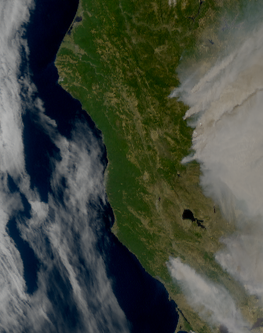
The event featured is the August Complex fire in California, USA in 2020. This was the largest wildfire in CA history, spreading over 1,000,000 acres (over 4,000 sq km). The image shown in this notebook is taken from 7 October 2020.
Basic Facts
Spatial resolution: 500m
Spatial coverage: Western Hemisphere
Scan time: 5 to 15 minutes depending on mode
Data availability: since 2016
How to access the data
There are multiple ways to access the GOES-17 ABI data including from Amazon Web Services and Google Cloud Platform. You can manually download data from this Amazon Download Page created by Brian Blaylock. The data are distributed in netcdf format.
Load required libraries
import os
import xarray as xr
import numpy as np
import glob

from datetime import datetime
import pyresample as prs
from pyresample import get_area_def

from satpy.scene import Scene
from satpy import MultiScene
from satpy.writers import to_image
from satpy import find_files_and_readers

import imageio_ffmpeg
import pydecorate

from IPython.display import Video

import warnings
import logging
warnings.filterwarnings('ignore')
warnings.simplefilter(action = "ignore", category = RuntimeWarning)
logging.basicConfig(level=logging.ERROR)
Load and browse GOES-17 ABI Level 1B Calibrated Radiances data
GOES-17 ABI data is disseminated in the netcdf format. You will use the Python library satpy to open the data. The results in a netCDF4.Dataset, which contains the dataset’s metadata, dimension and variable information.
Read more about satpy here.
From the Amazon Download Page, you can download Level-1B data for every available band on 20 August 2021 for every 10 minutes from 20:01 to 22:51 UTC. The data is available in the folder ../data/goes/17/level1b/2020/08/20. Let us load the data. First, you specify the file path and create a variable with the name file_name. Each file contains data from a single band.
Let us begin by visualizing data from a single time step from 20 August 2021 at 22:01 UTC.
file_name = glob.glob('../data/goes/17/level1b/2020/08/20/*e2020233220*.nc')
file_name
['../data/goes/17/level1b/2020/08/20/OR_ABI-L1b-RadC-M6C09_G17_s20202332201177_e20202332203556_c20202332204067.nc',
 '../data/goes/17/level1b/2020/08/20/OR_ABI-L1b-RadC-M6C06_G17_s20202332201177_e20202332203555_c20202332204010.nc',
 '../data/goes/17/level1b/2020/08/20/OR_ABI-L1b-RadC-M6C14_G17_s20202332201177_e20202332203550_c20202332204048.nc',
 '../data/goes/17/level1b/2020/08/20/OR_ABI-L1b-RadC-M6C08_G17_s20202332201177_e20202332203549_c20202332204062.nc',
 '../data/goes/17/level1b/2020/08/20/OR_ABI-L1b-RadC-M6C02_G17_s20202332201177_e20202332203550_c20202332203573.nc',
 '../data/goes/17/level1b/2020/08/20/OR_ABI-L1b-RadC-M6C05_G17_s20202332201177_e20202332203550_c20202332204004.nc',
 '../data/goes/17/level1b/2020/08/20/OR_ABI-L1b-RadC-M6C03_G17_s20202332201177_e20202332203550_c20202332203597.nc',
 '../data/goes/17/level1b/2020/08/20/OR_ABI-L1b-RadC-M6C01_G17_s20202332201177_e20202332203550_c20202332203579.nc',
 '../data/goes/17/level1b/2020/08/20/OR_ABI-L1b-RadC-M6C13_G17_s20202332201177_e20202332203561_c20202332204080.nc',
 '../data/goes/17/level1b/2020/08/20/OR_ABI-L1b-RadC-M6C12_G17_s20202332201177_e20202332203555_c20202332204016.nc',
 '../data/goes/17/level1b/2020/08/20/OR_ABI-L1b-RadC-M6C11_G17_s20202332201177_e20202332203549_c20202332204038.nc',
 '../data/goes/17/level1b/2020/08/20/OR_ABI-L1b-RadC-M6C15_G17_s20202332201177_e20202332203555_c20202332204075.nc',
 '../data/goes/17/level1b/2020/08/20/OR_ABI-L1b-RadC-M6C16_G17_s20202332201177_e20202332203561_c20202332204056.nc',
 '../data/goes/17/level1b/2020/08/20/OR_ABI-L1b-RadC-M6C07_G17_s20202332201177_e20202332203561_c20202332204024.nc',
 '../data/goes/17/level1b/2020/08/20/OR_ABI-L1b-RadC-M6C04_G17_s20202332201177_e20202332203549_c20202332203589.nc',
 '../data/goes/17/level1b/2020/08/20/OR_ABI-L1b-RadC-M6C10_G17_s20202332201177_e20202332203562_c20202332204031.nc']
In a next step, you use the Scene constructor from the satpy library. Once loaded, a Scene object represents a single geographic region of data, typically at a single continuous time range.
You have to specify the two keyword arguments reader and filenames in order to successfully load a scene. As mentioned above, for GOES-17 Level-1B data, you can use the abi_l1b reader.
scn =Scene(filenames=file_name,reader='abi_l1b')

scn
<satpy.scene.Scene at 0x7f38803a1700>
A Scene object is a collection of different bands, with the function available_dataset_names(), you can see the available bands of the scene. To learn more about the bands of GOES-17, visit this website.
scn.available_dataset_names()
['C01',
 'C02',
 'C03',
 'C04',
 'C05',
 'C06',
 'C07',
 'C08',
 'C09',
 'C10',
 'C11',
 'C12',
 'C13',
 'C14',
 'C15',
 'C16']
The underlying container for data in satpy is the xarray.DataArray. With the function load(), you can specify an individual band by name, e.g. C01 and load the data. If you then select the loaded band, you see that the band object is a xarray.DataArray.
scn.load(['C01'])
scn['C01']
<xarray.DataArray (y: 3000, x: 5000)>
dask.array<mul, shape=(3000, 5000), dtype=float64, chunksize=(3000, 4096), chunktype=numpy.ndarray>
Coordinates:
    crs      object PROJCRS["unknown",BASEGEOGCRS["unknown",DATUM["unknown",E...
  * y        (y) float64 4.589e+06 4.588e+06 4.587e+06 ... 1.585e+06 1.584e+06
  * x        (x) float64 -2.505e+06 -2.504e+06 ... 2.504e+06 2.505e+06
Attributes:
    orbital_parameters:     {'projection_longitude': -137.0, 'projection_lati...
    long_name:              Bidirectional Reflectance
    standard_name:          toa_bidirectional_reflectance
    sensor_band_bit_depth:  10
    units:                  %
    resolution:             1000
    grid_mapping:           goes_imager_projection
    cell_methods:           t: point area: point
    platform_name:          GOES-17
    sensor:                 abi
    name:                   C01
    wavelength:             0.47 µm (0.45-0.49 µm)
    calibration:            reflectance
    modifiers:              ()
    observation_type:       Rad
    scene_abbr:             C
    scan_mode:              M6
    platform_shortname:     G17
    scene_id:               CONUS
    orbital_slot:           GOES-West
    instrument_ID:          FM2
    production_site:        WCDAS
    timeline_ID:            None
    start_time:             2020-08-20 22:01:17.700000
    end_time:               2020-08-20 22:03:55
    reader:                 abi_l1b
    area:                   Area ID: GOES-West\nDescription: 1km at nadir\nPr...
    _satpy_id:              DataID(name='C01', wavelength=WavelengthRange(min...
ancillary_variables: []- y: 3000
- x: 5000
- dask.array<chunksize=(3000, 4096), meta=np.ndarray>
Array Chunk Bytes 114.44 MiB 93.75 MiB Shape (3000, 5000) (3000, 4096) Count 20 Tasks 2 Chunks Type float64 numpy.ndarray - crs()objectPROJCRS["unknown",BASEGEOGCRS["u...
array(<Projected CRS: PROJCRS["unknown",BASEGEOGCRS["unknown",DATUM["unk ...>
Name: unknown
Axis Info [cartesian]:
- E[east]: Easting (metre)
- N[north]: Northing (metre)
Area of Use:
- undefined
Coordinate Operation:
- name: unknown
- method: Geostationary Satellite (Sweep X)
Datum: unknown
- Ellipsoid: GRS 1980
- Prime Meridian: Greenwich
, dtype=object)
- y(y)float644.589e+06 4.588e+06 ... 1.584e+06
- units :
- meter
array([4588698.585198, 4587696.576554, 4586694.56791 , ..., 1585678.67913 , 1584676.670486, 1583674.661842]) - x(x)float64-2.505e+06 -2.504e+06 ... 2.505e+06
- units :
- meter
array([-2504520.605678, -2503518.597034, -2502516.58839 , ...,  2502516.58839 ,
        2503518.597034,  2504520.605678])
- orbital_parameters :
- {'projection_longitude': -137.0, 'projection_latitude': 0.0, 'projection_altitude': 35786023.0, 'satellite_nominal_latitude': 0.0, 'satellite_nominal_longitude': -137.1999969482422, 'satellite_nominal_altitude': 35786023.4375, 'yaw_flip': False}
- long_name :
- Bidirectional Reflectance
- standard_name :
- toa_bidirectional_reflectance
- sensor_band_bit_depth :
- 10
- units :
- %
- resolution :
- 1000
- grid_mapping :
- goes_imager_projection
- cell_methods :
- t: point area: point
- platform_name :
- GOES-17
- sensor :
- abi
- name :
- C01
- wavelength :
- 0.47 µm (0.45-0.49 µm)
- calibration :
- reflectance
- modifiers :
- ()
- observation_type :
- Rad
- scene_abbr :
- C
- scan_mode :
- M6
- platform_shortname :
- G17
- scene_id :
- CONUS
- orbital_slot :
- GOES-West
- instrument_ID :
- FM2
- production_site :
- WCDAS
- timeline_ID :
- None
- start_time :
- 2020-08-20 22:01:17.700000
- end_time :
- 2020-08-20 22:03:55
- reader :
- abi_l1b
- area :
- Area ID: GOES-West Description: 1km at nadir Projection ID: abi_fixed_grid Projection: {'ellps': 'GRS80', 'h': '35786023', 'lon_0': '-137', 'no_defs': 'None', 'proj': 'geos', 'sweep': 'x', 'type': 'crs', 'units': 'm', 'x_0': '0', 'y_0': '0'} Number of columns: 5000 Number of rows: 3000 Area extent: (-2505021.61, 1583173.6575, 2505021.61, 4589199.5895)
- _satpy_id :
- DataID(name='C01', wavelength=WavelengthRange(min=0.45, central=0.47, max=0.49, unit='µm'), resolution=1000, calibration=<calibration.reflectance>, modifiers=())
- ancillary_variables :
- []
With an xarray data structure, you can handle the object as a xarray.DataArray. For example, you can print a list of available attributes with the function attrs.keys().
scn['C01'].attrs.keys()
dict_keys(['orbital_parameters', 'long_name', 'standard_name', 'sensor_band_bit_depth', 'units', 'resolution', 'grid_mapping', 'cell_methods', 'platform_name', 'sensor', 'name', 'wavelength', 'calibration', 'modifiers', 'observation_type', 'scene_abbr', 'scan_mode', 'platform_shortname', 'scene_id', 'orbital_slot', 'instrument_ID', 'production_site', 'timeline_ID', 'start_time', 'end_time', 'reader', 'area', '_satpy_id', 'ancillary_variables'])
With the attrs() function, you can also access individual metadata information, e.g. start_time and end_time.
scn['C01'].attrs['start_time'], scn['C01'].attrs['end_time']
(datetime.datetime(2020, 8, 20, 22, 1, 17, 700000),
 datetime.datetime(2020, 8, 20, 22, 3, 55))
Browse and visualize composite IDs
composites combine three window channel of satellite data in order to get e.g. a true-color image of the scene. Depending on which channel combination is used, different features can be highlighted in the composite, e.g. dust. The satpy library offers several predefined composites options. The function available_composite_ids() returns a list of available composite IDs.
scn.available_composite_ids()
[DataID(name='airmass'),
 DataID(name='ash'),
 DataID(name='cimss_cloud_type'),
 DataID(name='cimss_green'),
 DataID(name='cimss_green_sunz'),
 DataID(name='cimss_green_sunz_rayleigh'),
 DataID(name='cimss_true_color'),
 DataID(name='cimss_true_color_sunz'),
 DataID(name='cimss_true_color_sunz_rayleigh'),
 DataID(name='cira_day_convection'),
 DataID(name='cira_fire_temperature'),
 DataID(name='cloud_phase'),
 DataID(name='cloud_phase_distinction'),
 DataID(name='cloud_phase_distinction_raw'),
 DataID(name='cloud_phase_raw'),
 DataID(name='cloudtop'),
 DataID(name='color_infrared'),
 DataID(name='colorized_ir_clouds'),
 DataID(name='convection'),
 DataID(name='day_microphysics'),
 DataID(name='day_microphysics_abi'),
 DataID(name='day_microphysics_eum'),
 DataID(name='dust'),
 DataID(name='fire_temperature_awips'),
 DataID(name='fog'),
 DataID(name='green'),
 DataID(name='green_crefl'),
 DataID(name='green_nocorr'),
 DataID(name='green_raw'),
 DataID(name='green_snow'),
 DataID(name='highlight_C14'),
 DataID(name='ir108_3d'),
 DataID(name='ir_cloud_day'),
 DataID(name='land_cloud'),
 DataID(name='land_cloud_fire'),
 DataID(name='natural_color'),
 DataID(name='natural_color_nocorr'),
 DataID(name='natural_color_raw'),
 DataID(name='night_fog'),
 DataID(name='night_ir_alpha'),
 DataID(name='night_ir_with_background'),
 DataID(name='night_ir_with_background_hires'),
 DataID(name='night_microphysics'),
 DataID(name='night_microphysics_abi'),
 DataID(name='overview'),
 DataID(name='overview_raw'),
 DataID(name='snow'),
 DataID(name='snow_fog'),
 DataID(name='so2'),
 DataID(name='tropical_airmass'),
 DataID(name='true_color'),
 DataID(name='true_color_crefl'),
 DataID(name='true_color_nocorr'),
 DataID(name='true_color_raw'),
 DataID(name='true_color_with_night_ir'),
 DataID(name='true_color_with_night_ir_hires'),
 DataID(name='water_vapors1'),
 DataID(name='water_vapors2')]
Let us define a list with a single element, true_color, to create a composite that visualize both the active fires as well as smoke. The fire which will be shown is the Doe Fire, which was a part of the August Complex fires.
This list (composite_id) can then be passed to the function load(). Per default, scenes are loaded with the north pole facing downwards. You can specify the keyword argument upper_right_corner=NE in order to turn the image around and have the north pole facing upwards.
composite_id = ['true_color']
scn.load(composite_id, upper_right_corner='NE')
Generate a geographical subset around northern California
Let us generate a geographical subset around northern California. You can do this with the function stored in the coord2area_def.py script which converts human coordinates (longitude and latitude) to an area definition.
You need to define the following arguments:
name:the name of the area definition, set this tocalifornia_500mproj: the projection, set this tolaeawhich stands for the Lambert azimuthal equal-area projectionmin_lat: the minimum latitude value, set this to38max_lat: the maximum latitude value, set this to41min_lon: the minimum longitude value, set this to-125max_lon: the maximum longitude value, set this to-122resolution(km): the resolution in kilometres, set this to0.5
Afterwards, you can visualize the resampled image with the function show().
%run coord2area_def.py california_500m laea 38 41 -125 -122 0.5
### +proj=laea +lat_0=39.5 +lon_0=-123.5 +ellps=WGS84

california_500m:
  description: california_500m
  projection:
    proj: laea
    ellps: WGS84
    lat_0: 39.5
    lon_0: -123.5
  shape:
    height: 666
    width: 527
  area_extent:
    lower_left_xy: [-131748.033787, -165429.793658]
    upper_right_xy: [131748.033787, 167607.077655]
From the values generated by coord2area_def.py, you copy and paste several into the template below.
You need to define the following arguments in the code block template below:
area_id(string): the name of the area definition, set this to'california_500m'x_size(integer): the number of values for the width, set this to the value of the shapewidth, which is527y_size(integer): the number of values for the height, set this to the value of the shapeheight, which is666area_extent(set of coordinates in brackets): the extent of the map is defined by 2 sets of coordinates, within a set of brackets()paste in the values of thelower_left_xyfrom the area_extent above, followed by theupper_right_xyvalues. You should end up with(-131748.033787, -165429.793658, 131748.033787, 167607.077655).projection(string): the projection, paste in the first line after###starting with+proj, e.g.'+proj=laea +lat_0=39.5 +lon_0=-123.5 +ellps=WGS84'description(string): Give this a generic name for the region, such as'California'proj_id(string): A recommended format is the projection short code followed by lat_0 and lon_0, e.g.'laea_39.5_-123.5'
Next, use the area definition to resample the loaded Scene object. You will make use of the get_area_def function from the pyresample library.
You should end up with the following code block.
area_id = 'california_500m'

x_size = 527
y_size = 666
area_extent = (-131748.033787, -165429.793658, 131748.033787, 167607.077655)
projection = '+proj=laea +lat_0=39.5 +lon_0=-123.5 +ellps=WGS84'
description = "California"
proj_id = 'laea_39.5_-123.5'

areadef = get_area_def(area_id, description, proj_id, projection,x_size, y_size, area_extent)
Next, use the area definition to resample the loaded Scene object.
scn_resample = scn.resample(areadef)
Afterwards, you can visualize the resampled image with the function show().
scn_resample.show('true_color')
Create time-lapse animation of true colour composite imagery
Next, you can create a time-lapse animation of the true colour composite imagery using the satpy library. You begin by first defining the folder path to the base directory where the data files are stored.
folder_path = '../data/goes/17/level1b/2020/08/20/'
You can create a MultiScene object from all the files in the base directory, using the abi_l1b reader.
from glob import glob
mscn = MultiScene.from_files(glob(os.path.join(folder_path, 'OR_*.nc')), reader='abi_l1b')
Then, you load the true colour composite for this MultiScene object using the .load() function.
mscn.load(['true_color'])
Finally you can resample the MultiScene object by the area definition you defined earlier which is stored in the variable areadef.
new_mscn = mscn.resample(areadef)
If you want to save this animation, you can uncomment the following codeblock to save it as an mpeg4 file.
# new_mscn.save_animation('{name}_{start_time:%Y%m%d_%H%M%S}.mp4', fps=5)
Now, we have saved and exported an animation video beforehand. You can view the video using the Video function from iPython.display.
Video('./img/true_color_20200820_200117.mp4', width=500, height=500)
Create an animation with text
To add text to the video, you can use the imageio-ffmpeg and the pydecorate libraries. Note that creating this video could take ten minutes or longer. To create and save the animation, you can remove the """ blockquotes from the following code block.
You can reuse the resampled MultiScene object that you created earlier, which is stored in the variable new_mscn.
First, set the file name of the mpeg4 file. This is formatted as text_{name:s}_{start_time:%Y%m%d_%H%M}.mp4, which will result in a file name of text_true_color_20200820_2001.mp4
You can define the text that will appear in the video by changing the txt value. This is currently set as California, USA {start_time:%Y-%m-%d %H:%M} showing the location as well as the date and time that the image was recorded.
You can align the text to one of the corners of the image by changing the values of top_bottom and left_right. We have aligned the text to appear on the top-left by setting the value of top_bottom to "top" and the value of left_right to "left"
You will need to also provide the file-path to a .ttf font file. We are using an open source font called SourceSansPro-Bold.
The final parameters you can change are:
font_size: the size of the fontheight: the height of the text boxbg: the background colour of the text boxbg_opacity: the opacity of the text boxline: the color of the linefps: the number of frames per second
"""
new_mscn.save_animation(
    "text_{name:s}_{start_time:%Y%m%d_%H%M}.mp4",
    enh_args={
    "decorate": {
        "decorate": [
            {"text": {
                "txt": "California, USA {start_time:%Y-%m-%d %H:%M}",
                "align": {
                    "top_bottom": "top",
                    "left_right": "left"},
                "font": '../data/goes/17/level1b/2020/08/20/SourceSansPro-Bold.ttf',
                "font_size": 20,
                "height": 30,
                "bg": "black",
                "bg_opacity": 255,
                "line": "white"}}]}},
    fps=5
)
"""
Now, we have saved and exported an animation video with text beforehand. You can view the video using the Video function from iPython.display.
Video('./img/text_true_color_20200820_2001.mp4', width=500, height=500)
References
GOES-R Calibration Working Group and GOES-R Series Program. (2017). NOAA GOES-R Series Advanced Baseline Imager (ABI) Level 1b Radiances. NOAA National Centers for Environmental Information. doi:10.7289/V5BV7DSR.
Some code in this notebook was adapted from the following source:
origin: https://satpy.readthedocs.io/en/stable/multiscene.html#saving-frames-of-an-animation
copyright: 2009-2022, Pytroll developers
license: GPL-3.0 License
retrieved: 2022-06-28 by Sabrina Szeto
Return to the case study
Monitoring fires with next-generation satellites from MTG and Metop-SG: Californian Wildfires Case Study
True colour composite imagery