Copernicus Sentinel-5P TROPOMI - Carbon Monoxide - Level 2
Contents
Copernicus Sentinel-5P TROPOMI - Carbon Monoxide - Level 2
The Copernicus Sentinel-5 Ultraviolet Visible Near-Infrared Shortwave (UVNS) spectrometer enables the measurement of trace gases which will improve air quality forecasts produced by the Copernicus Atmosphere Monitoring service.
This notebook provides you an introduction to data from Sentinel-5P, the precursor instrument and proxy for data from Sentinel-5.
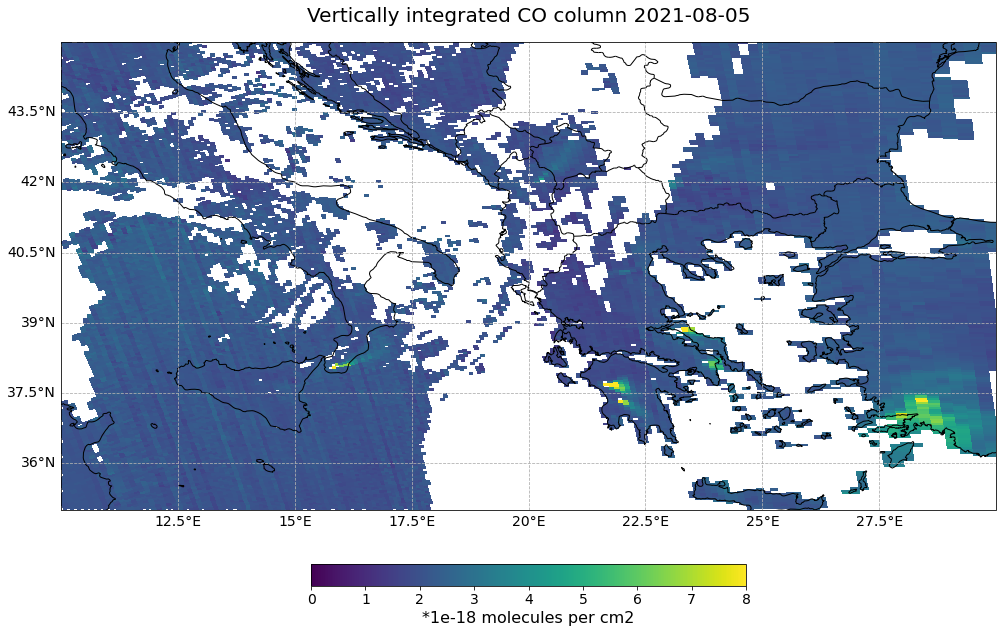
The data product of interest is the total column of carbon monoxide sensed by Sentinel-5P TROPOMI. Carbon monoxide is a good trace gas for monitoring and tracking smoke from wildfires.
The events featured in this notebook are the wildfires in Italy and Greece in summer 2021.
Basic Facts
Spatial resolution: Up to 5.5* km x 3.5 km (5.5 km in the satellite flight direction and 3.5 km in the perpendicular direction at nadir)
Spatial coverage: Global
Revisit time: less than one day
Data availability: since April 2018
How to access the data
Sentinel-5P Pre-Ops data are disseminated in the netCDF format and can be downloaded via the Copernicus Open Access Hub. You need to register for an account before downloading data.
Load required libraries
import os
import xarray as xr
import numpy as np
import netCDF4 as nc

# Python libraries for visualization
%matplotlib inline
import matplotlib.pyplot as plt
from matplotlib.axes import Axes
import cartopy.crs as ccrs
from cartopy.mpl.gridliner import LONGITUDE_FORMATTER, LATITUDE_FORMATTER
import cartopy.feature as cfeature
from cartopy.mpl.geoaxes import GeoAxes
GeoAxes._pcolormesh_patched = Axes.pcolormesh

import warnings
import logging
warnings.filterwarnings('ignore')
warnings.simplefilter(action = "ignore", category = RuntimeWarning)
logging.basicConfig(level=logging.ERROR)
Load helper functions
%run ../functions.ipynb
Load and browse Sentinel-5P TROPOMI Carbon Monoxide Level 2 data
A Sentinel-5P TROPOMI Carbon Monoxide Level 2 file is organised in two groups: PRODUCT and METADATA. The PRODUCT group stores the main data fields of the product, including latitude, longitude and the variable itself. The METADATA group provides additional metadata items.
Sentinel-5P TROPOMI variables have the following dimensions:
scanline: the number of measurements in the granule / along-track dimension indexground_pixel: the number of spectra in a measurement / across-track dimension indextime: time reference for the datacorner: pixel corner indexlayer: this dimension indicates the vertical grid of profile variables
Sentinel-5P TROPOMI data is disseminated in netCDF. You can load a netCDF file with the open_dataset() function of the xarray library. In order to load the variable as part of a Sentinel-5P data files, you have to specify the following keyword arguments:
group='PRODUCT': to load thePRODUCTgroup.
Let us load a Sentinel-5P TROPOMI data file as xarray.Dataset from 05 August 2021 and inspect the data structure:
s5p = xr.open_dataset('../data/sentinel-5p/co/2021/08/05/S5P_OFFL_L2__CO_____20210805T110012_20210805T124141_19750_02_020200_20210807T004645.nc', group='PRODUCT')
s5p
<xarray.Dataset>
Dimensions:                                (scanline: 4172, ground_pixel: 215, time: 1, corner: 4, layer: 50)
Coordinates:
  * scanline                               (scanline) float64 0.0 ... 4.171e+03
  * ground_pixel                           (ground_pixel) float64 0.0 ... 214.0
  * time                                   (time) datetime64[ns] 2021-08-05
  * corner                                 (corner) float64 0.0 1.0 2.0 3.0
  * layer                                  (layer) float32 4.95e+04 ... 500.0
    latitude                               (time, scanline, ground_pixel) float32 ...
    longitude                              (time, scanline, ground_pixel) float32 ...
Data variables:
    delta_time                             (time, scanline) datetime64[ns] 20...
    time_utc                               (time, scanline) object '2021-08-0...
    qa_value                               (time, scanline, ground_pixel) float32 ...
    carbonmonoxide_total_column            (time, scanline, ground_pixel) float32 ...
    carbonmonoxide_total_column_precision  (time, scanline, ground_pixel) float32 ...
carbonmonoxide_total_column_corrected (time, scanline, ground_pixel) float32 ...- scanline: 4172
- ground_pixel: 215
- time: 1
- corner: 4
- layer: 50
- scanline(scanline)float640.0 1.0 2.0 ... 4.17e+03 4.171e+03
- units :
- 1
- axis :
- Y
- long_name :
- along-track dimension index
- comment :
- This coordinate variable defines the indices along track; index starts at 0
array([0.000e+00, 1.000e+00, 2.000e+00, ..., 4.169e+03, 4.170e+03, 4.171e+03])
- ground_pixel(ground_pixel)float640.0 1.0 2.0 ... 212.0 213.0 214.0
- units :
- 1
- axis :
- X
- long_name :
- across-track dimension index
- comment :
- This coordinate variable defines the indices across track, from west to east; index starts at 0
array([ 0., 1., 2., ..., 212., 213., 214.])
- time(time)datetime64[ns]2021-08-05
- standard_name :
- time
- axis :
- T
- long_name :
- reference time for the measurements
- comment :
- The time in this variable corresponds to the time in the time_reference global attribute
array(['2021-08-05T00:00:00.000000000'], dtype='datetime64[ns]')
- corner(corner)float640.0 1.0 2.0 3.0
- units :
- 1
- long_name :
- pixel corner index
- comment :
- This coordinate variable defines the indices for the pixel corners; index starts at 0 (counter-clockwise, starting from south-western corner of the pixel in ascending part of the orbit)
array([0., 1., 2., 3.])
- layer(layer)float324.95e+04 4.85e+04 ... 1.5e+03 500.0
- units :
- m
- standard_name :
- height
- long_name :
- Height above topographic surface
- axis :
- Z
array([49500., 48500., 47500., 46500., 45500., 44500., 43500., 42500., 41500., 40500., 39500., 38500., 37500., 36500., 35500., 34500., 33500., 32500., 31500., 30500., 29500., 28500., 27500., 26500., 25500., 24500., 23500., 22500., 21500., 20500., 19500., 18500., 17500., 16500., 15500., 14500., 13500., 12500., 11500., 10500., 9500., 8500., 7500., 6500., 5500., 4500., 3500., 2500., 1500., 500.], dtype=float32) - latitude(time, scanline, ground_pixel)float32...
- long_name :
- pixel center latitude
- units :
- degrees_north
- standard_name :
- latitude
- valid_min :
- -90.0
- valid_max :
- 90.0
- bounds :
- /PRODUCT/SUPPORT_DATA/GEOLOCATIONS/latitude_bounds
[896980 values with dtype=float32]
- longitude(time, scanline, ground_pixel)float32...
- long_name :
- pixel center longitude
- units :
- degrees_east
- standard_name :
- longitude
- valid_min :
- -180.0
- valid_max :
- 180.0
- bounds :
- /PRODUCT/SUPPORT_DATA/GEOLOCATIONS/longitude_bounds
[896980 values with dtype=float32]
- delta_time(time, scanline)datetime64[ns]...
- long_name :
- offset of start time of measurement relative to time_reference
array([['2021-08-05T11:21:47.151000000', '2021-08-05T11:21:47.991000000', '2021-08-05T11:21:48.831000000', ..., '2021-08-05T12:20:09.030000000', '2021-08-05T12:20:09.870000000', '2021-08-05T12:20:10.710000000']], dtype='datetime64[ns]') - time_utc(time, scanline)object...
- long_name :
- Time of observation as ISO 8601 date-time string
array([['2021-08-05T11:21:47.151000Z', '2021-08-05T11:21:47.991000Z', '2021-08-05T11:21:48.831000Z', ..., '2021-08-05T12:20:09.030000Z', '2021-08-05T12:20:09.870000Z', '2021-08-05T12:20:10.710000Z']], dtype=object) - qa_value(time, scanline, ground_pixel)float32...
- units :
- 1
- valid_min :
- 0
- valid_max :
- 100
- long_name :
- data quality value
- comment :
- A continuous quality descriptor, varying between 0 (no data) and 1 (full quality data). Recommend to ignore data with qa_value < 0.5
[896980 values with dtype=float32]
- carbonmonoxide_total_column(time, scanline, ground_pixel)float32...
- units :
- mol m-2
- standard_name :
- atmosphere_mole_content_of_carbon_monoxide
- long_name :
- Vertically integrated CO column
- ancillary_variables :
- carbonmonoxide_total_column_precision
- multiplication_factor_to_convert_to_molecules_percm2 :
- 6.022141e+19
[896980 values with dtype=float32]
- carbonmonoxide_total_column_precision(time, scanline, ground_pixel)float32...
- units :
- mol m-2
- standard_name :
- atmosphere_mole_content_of_carbon_monoxide standard_error
- long_name :
- Standard error of the vertically integrated CO column
- multiplication_factor_to_convert_to_molecules_percm2 :
- 6.022141e+19
[896980 values with dtype=float32]
- carbonmonoxide_total_column_corrected(time, scanline, ground_pixel)float32...
- units :
- mol m-2
- standard_name :
- atmosphere_mole_content_of_carbon_monoxide
- long_name :
- carbonmonoxide_total_column - carbonmonoxide_total_column_stripe_offset
- ancillary_variables :
- carbonmonoxide_total_column_precision carbonmonoxide_total_column_stripe_offset
- multiplication_factor_to_convert_to_molecules_percm2 :
- 6.022141e+19
[896980 values with dtype=float32]
You see that the loaded data object contains of five dimensions and five data variables:
Dimensions:
scanlineground_pixeltimecornerlayer
Data variables:
delta_time: the offset of individual measurements within the granule, given in millisecondstime_utc: valid time stamp of the dataga_value: quality descriptor, varying between 0 (nodata) and 1 (full quality data).carbonmonoxide_total_column: Vertically integrated CO column densitycarbonmonoxide_total_column_precision: Standard error of the vertically integrate CO column
You can specify one variable of interest by putting the name of the variable into square brackets [] and get more detailed information about the variable. E.g. carbonmonoxide_total_column is the atmosphere mole content of carbon monoxide, has the unit mol per m-2, and has three dimensions, time, scanline and groundpixel respectively.
s5p_co = s5p['carbonmonoxide_total_column']
s5p_co
<xarray.DataArray 'carbonmonoxide_total_column' (time: 1, scanline: 4172, ground_pixel: 215)>
[896980 values with dtype=float32]
Coordinates:
  * scanline      (scanline) float64 0.0 1.0 2.0 ... 4.17e+03 4.171e+03
  * ground_pixel  (ground_pixel) float64 0.0 1.0 2.0 3.0 ... 212.0 213.0 214.0
  * time          (time) datetime64[ns] 2021-08-05
    latitude      (time, scanline, ground_pixel) float32 ...
    longitude     (time, scanline, ground_pixel) float32 ...
Attributes:
    units:                                                 mol m-2
    standard_name:                                         atmosphere_mole_co...
    long_name:                                             Vertically integra...
    ancillary_variables:                                   carbonmonoxide_tot...
multiplication_factor_to_convert_to_molecules_percm2: 6.022141e+19- time: 1
- scanline: 4172
- ground_pixel: 215
- ...
[896980 values with dtype=float32]
- scanline(scanline)float640.0 1.0 2.0 ... 4.17e+03 4.171e+03
- units :
- 1
- axis :
- Y
- long_name :
- along-track dimension index
- comment :
- This coordinate variable defines the indices along track; index starts at 0
array([0.000e+00, 1.000e+00, 2.000e+00, ..., 4.169e+03, 4.170e+03, 4.171e+03])
- ground_pixel(ground_pixel)float640.0 1.0 2.0 ... 212.0 213.0 214.0
- units :
- 1
- axis :
- X
- long_name :
- across-track dimension index
- comment :
- This coordinate variable defines the indices across track, from west to east; index starts at 0
array([ 0., 1., 2., ..., 212., 213., 214.])
- time(time)datetime64[ns]2021-08-05
- standard_name :
- time
- axis :
- T
- long_name :
- reference time for the measurements
- comment :
- The time in this variable corresponds to the time in the time_reference global attribute
array(['2021-08-05T00:00:00.000000000'], dtype='datetime64[ns]')
- latitude(time, scanline, ground_pixel)float32...
- long_name :
- pixel center latitude
- units :
- degrees_north
- standard_name :
- latitude
- valid_min :
- -90.0
- valid_max :
- 90.0
- bounds :
- /PRODUCT/SUPPORT_DATA/GEOLOCATIONS/latitude_bounds
[896980 values with dtype=float32]
- longitude(time, scanline, ground_pixel)float32...
- long_name :
- pixel center longitude
- units :
- degrees_east
- standard_name :
- longitude
- valid_min :
- -180.0
- valid_max :
- 180.0
- bounds :
- /PRODUCT/SUPPORT_DATA/GEOLOCATIONS/longitude_bounds
[896980 values with dtype=float32]
- units :
- mol m-2
- standard_name :
- atmosphere_mole_content_of_carbon_monoxide
- long_name :
- Vertically integrated CO column
- ancillary_variables :
- carbonmonoxide_total_column_precision
- multiplication_factor_to_convert_to_molecules_percm2 :
- 6.022141e+19
You can do this for the available variables, but also for the dimensions latitude and longitude.
print('Latitude')
print(s5p_co.latitude)

print('Longitude')
print(s5p_co.longitude)
Latitude
<xarray.DataArray 'latitude' (time: 1, scanline: 4172, ground_pixel: 215)>
[896980 values with dtype=float32]
Coordinates:
  * scanline      (scanline) float64 0.0 1.0 2.0 ... 4.17e+03 4.171e+03
  * ground_pixel  (ground_pixel) float64 0.0 1.0 2.0 3.0 ... 212.0 213.0 214.0
  * time          (time) datetime64[ns] 2021-08-05
    latitude      (time, scanline, ground_pixel) float32 ...
    longitude     (time, scanline, ground_pixel) float32 ...
Attributes:
    long_name:      pixel center latitude
    units:          degrees_north
    standard_name:  latitude
    valid_min:      -90.0
    valid_max:      90.0
    bounds:         /PRODUCT/SUPPORT_DATA/GEOLOCATIONS/latitude_bounds
Longitude
<xarray.DataArray 'longitude' (time: 1, scanline: 4172, ground_pixel: 215)>
[896980 values with dtype=float32]
Coordinates:
  * scanline      (scanline) float64 0.0 1.0 2.0 ... 4.17e+03 4.171e+03
  * ground_pixel  (ground_pixel) float64 0.0 1.0 2.0 3.0 ... 212.0 213.0 214.0
  * time          (time) datetime64[ns] 2021-08-05
    latitude      (time, scanline, ground_pixel) float32 ...
    longitude     (time, scanline, ground_pixel) float32 ...
Attributes:
    long_name:      pixel center longitude
    units:          degrees_east
    standard_name:  longitude
    valid_min:      -180.0
    valid_max:      180.0
    bounds:         /PRODUCT/SUPPORT_DATA/GEOLOCATIONS/longitude_bounds
You can retrieve the array values of the variable with squared brackets: [:,:,:]. One single time step can be selected by specifying one value of the time dimension, e.g. [0,:,:].
s5p_co_0708 = s5p_co[0,:,:]
s5p_co_0708
<xarray.DataArray 'carbonmonoxide_total_column' (scanline: 4172, ground_pixel: 215)>
[896980 values with dtype=float32]
Coordinates:
  * scanline      (scanline) float64 0.0 1.0 2.0 ... 4.17e+03 4.171e+03
  * ground_pixel  (ground_pixel) float64 0.0 1.0 2.0 3.0 ... 212.0 213.0 214.0
    time          datetime64[ns] 2021-08-05
    latitude      (scanline, ground_pixel) float32 ...
    longitude     (scanline, ground_pixel) float32 ...
Attributes:
    units:                                                 mol m-2
    standard_name:                                         atmosphere_mole_co...
    long_name:                                             Vertically integra...
    ancillary_variables:                                   carbonmonoxide_tot...
multiplication_factor_to_convert_to_molecules_percm2: 6.022141e+19- scanline: 4172
- ground_pixel: 215
- ...
[896980 values with dtype=float32]
- scanline(scanline)float640.0 1.0 2.0 ... 4.17e+03 4.171e+03
- units :
- 1
- axis :
- Y
- long_name :
- along-track dimension index
- comment :
- This coordinate variable defines the indices along track; index starts at 0
array([0.000e+00, 1.000e+00, 2.000e+00, ..., 4.169e+03, 4.170e+03, 4.171e+03])
- ground_pixel(ground_pixel)float640.0 1.0 2.0 ... 212.0 213.0 214.0
- units :
- 1
- axis :
- X
- long_name :
- across-track dimension index
- comment :
- This coordinate variable defines the indices across track, from west to east; index starts at 0
array([ 0., 1., 2., ..., 212., 213., 214.])
- time()datetime64[ns]2021-08-05
- standard_name :
- time
- axis :
- T
- long_name :
- reference time for the measurements
- comment :
- The time in this variable corresponds to the time in the time_reference global attribute
array('2021-08-05T00:00:00.000000000', dtype='datetime64[ns]') - latitude(scanline, ground_pixel)float32...
- long_name :
- pixel center latitude
- units :
- degrees_north
- standard_name :
- latitude
- valid_min :
- -90.0
- valid_max :
- 90.0
- bounds :
- /PRODUCT/SUPPORT_DATA/GEOLOCATIONS/latitude_bounds
[896980 values with dtype=float32]
- longitude(scanline, ground_pixel)float32...
- long_name :
- pixel center longitude
- units :
- degrees_east
- standard_name :
- longitude
- valid_min :
- -180.0
- valid_max :
- 180.0
- bounds :
- /PRODUCT/SUPPORT_DATA/GEOLOCATIONS/longitude_bounds
[896980 values with dtype=float32]
- units :
- mol m-2
- standard_name :
- atmosphere_mole_content_of_carbon_monoxide
- long_name :
- Vertically integrated CO column
- ancillary_variables :
- carbonmonoxide_total_column_precision
- multiplication_factor_to_convert_to_molecules_percm2 :
- 6.022141e+19
The attributes of the xarray.DataArray hold the entry multiplication_factor_to_convert_to_molecules_percm2, which is a conversion factor that has to be applied to convert the data from mol per m2 to molecules per cm2.
conversion_factor = s5p_co.multiplication_factor_to_convert_to_molecules_percm2
conversion_factor
6.022141e+19
Additionally, you can save the attribute longname, which you can make use of when visualizing the data.
longname = s5p_co.long_name
longname
'Vertically integrated CO column'
Create a geographical subset around Italy and Greece
You can zoom into a region by specifying a bounding box of interest. Let us set the extent to Italy and Greece with the following bounding box information:
lonmin=10
lonmax=30
latmin=35
latmax=45
You can use the function generate_geographical_subsetto subset an xarray.DataArray based on a given bounding box.
s5p_co_subset = generate_geographical_subset(xarray=s5p_co_0708,
                                             latmin=latmin,
                                             latmax=latmax,
                                             lonmin=lonmin,
                                             lonmax=lonmax)
s5p_co_subset
<xarray.DataArray 'carbonmonoxide_total_column' (scanline: 241, ground_pixel: 179)>
array([[nan, nan, nan, ..., nan, nan, nan],
       [nan, nan, nan, ..., nan, nan, nan],
       [nan, nan, nan, ..., nan, nan, nan],
       ...,
       [nan, nan, nan, ..., nan, nan, nan],
       [nan, nan, nan, ..., nan, nan, nan],
       [nan, nan, nan, ..., nan, nan, nan]], dtype=float32)
Coordinates:
  * scanline      (scanline) float64 2.365e+03 2.366e+03 ... 2.604e+03 2.605e+03
  * ground_pixel  (ground_pixel) float64 33.0 34.0 35.0 ... 209.0 210.0 211.0
    time          datetime64[ns] 2021-08-05
    latitude      (scanline, ground_pixel) float32 32.2 32.24 ... 46.55 46.52
    longitude     (scanline, ground_pixel) float32 11.21 11.34 ... 29.3 29.69
Attributes:
    units:                                                 mol m-2
    standard_name:                                         atmosphere_mole_co...
    long_name:                                             Vertically integra...
    ancillary_variables:                                   carbonmonoxide_tot...
multiplication_factor_to_convert_to_molecules_percm2: 6.022141e+19- scanline: 241
- ground_pixel: 179
- nan nan nan nan nan nan nan nan ... nan nan nan nan nan nan nan nan
array([[nan, nan, nan, ..., nan, nan, nan], [nan, nan, nan, ..., nan, nan, nan], [nan, nan, nan, ..., nan, nan, nan], ..., [nan, nan, nan, ..., nan, nan, nan], [nan, nan, nan, ..., nan, nan, nan], [nan, nan, nan, ..., nan, nan, nan]], dtype=float32) - scanline(scanline)float642.365e+03 2.366e+03 ... 2.605e+03
- units :
- 1
- axis :
- Y
- long_name :
- along-track dimension index
- comment :
- This coordinate variable defines the indices along track; index starts at 0
array([2365., 2366., 2367., ..., 2603., 2604., 2605.])
- ground_pixel(ground_pixel)float6433.0 34.0 35.0 ... 210.0 211.0
- units :
- 1
- axis :
- X
- long_name :
- across-track dimension index
- comment :
- This coordinate variable defines the indices across track, from west to east; index starts at 0
array([ 33., 34., 35., 36., 37., 38., 39., 40., 41., 42., 43., 44., 45., 46., 47., 48., 49., 50., 51., 52., 53., 54., 55., 56., 57., 58., 59., 60., 61., 62., 63., 64., 65., 66., 67., 68., 69., 70., 71., 72., 73., 74., 75., 76., 77., 78., 79., 80., 81., 82., 83., 84., 85., 86., 87., 88., 89., 90., 91., 92., 93., 94., 95., 96., 97., 98., 99., 100., 101., 102., 103., 104., 105., 106., 107., 108., 109., 110., 111., 112., 113., 114., 115., 116., 117., 118., 119., 120., 121., 122., 123., 124., 125., 126., 127., 128., 129., 130., 131., 132., 133., 134., 135., 136., 137., 138., 139., 140., 141., 142., 143., 144., 145., 146., 147., 148., 149., 150., 151., 152., 153., 154., 155., 156., 157., 158., 159., 160., 161., 162., 163., 164., 165., 166., 167., 168., 169., 170., 171., 172., 173., 174., 175., 176., 177., 178., 179., 180., 181., 182., 183., 184., 185., 186., 187., 188., 189., 190., 191., 192., 193., 194., 195., 196., 197., 198., 199., 200., 201., 202., 203., 204., 205., 206., 207., 208., 209., 210., 211.]) - time()datetime64[ns]2021-08-05
- standard_name :
- time
- axis :
- T
- long_name :
- reference time for the measurements
- comment :
- The time in this variable corresponds to the time in the time_reference global attribute
array('2021-08-05T00:00:00.000000000', dtype='datetime64[ns]') - latitude(scanline, ground_pixel)float3232.2 32.24 32.29 ... 46.55 46.52
- long_name :
- pixel center latitude
- units :
- degrees_north
- standard_name :
- latitude
- valid_min :
- -90.0
- valid_max :
- 90.0
- bounds :
- /PRODUCT/SUPPORT_DATA/GEOLOCATIONS/latitude_bounds
array([[32.195065, 32.24469 , 32.293087, ..., 34.933292, 34.91955 , 34.90418 ], [32.2433 , 32.292946, 32.341362, ..., 34.981834, 34.968056, 34.952633], [32.291557, 32.341217, 32.389656, ..., 35.03038 , 35.016556, 35.001083], ..., [43.57638 , 43.632 , 43.686222, ..., 46.474236, 46.45017 , 46.423573], [43.623672, 43.679314, 43.73357 , ..., 46.522644, 46.498535, 46.47189 ], [43.670963, 43.726635, 43.78092 , ..., 46.571045, 46.546886, 46.520187]], dtype=float32) - longitude(scanline, ground_pixel)float3211.21 11.34 11.46 ... 29.3 29.69
- long_name :
- pixel center longitude
- units :
- degrees_east
- standard_name :
- longitude
- valid_min :
- -180.0
- valid_max :
- 180.0
- bounds :
- /PRODUCT/SUPPORT_DATA/GEOLOCATIONS/longitude_bounds
array([[11.211362 , 11.336978 , 11.460479 , ..., 30.425482 , 30.738092 ,
        31.064466 ],
       [11.193425 , 11.319099 , 11.442656 , ..., 30.418541 , 30.731333 ,
        31.057898 ],
       [11.1755085, 11.301239 , 11.424852 , ..., 30.411697 , 30.72468  ,
        31.051443 ],
       ...,
       [ 6.2271056,  6.3701506,  6.510907 , ..., 28.942106 , 29.31434  ,
        29.702757 ],
       [ 6.202429 ,  6.3455644,  6.4864106, ..., 28.936745 , 29.30931  ,
        29.698078 ],
       [ 6.1776867,  6.3209133,  6.4618506, ..., 28.931337 , 29.30424  ,
        29.693352 ]], dtype=float32)
- units :
- mol m-2
- standard_name :
- atmosphere_mole_content_of_carbon_monoxide
- long_name :
- Vertically integrated CO column
- ancillary_variables :
- carbonmonoxide_total_column_precision
- multiplication_factor_to_convert_to_molecules_percm2 :
- 6.022141e+19
Visualise Sentinel-5P TROPOMI Carbon Monoxide Level 2 data
You can plot data arrays of type numpy with matplotlib’s pcolormesh function. In combination with the library cartopy, you can produce high-quality maps.
In order to make it easier to visualize the Carbon Monoxide values, we apply the conversion factor to the xarray.DataArray. This converts the Carbon Monoxide values from mol per m2 to molecules per cm2.
s5p_co_converted = s5p_co_subset*conversion_factor
s5p_co_converted
<xarray.DataArray 'carbonmonoxide_total_column' (scanline: 241, ground_pixel: 179)>
array([[nan, nan, nan, ..., nan, nan, nan],
       [nan, nan, nan, ..., nan, nan, nan],
       [nan, nan, nan, ..., nan, nan, nan],
       ...,
       [nan, nan, nan, ..., nan, nan, nan],
       [nan, nan, nan, ..., nan, nan, nan],
       [nan, nan, nan, ..., nan, nan, nan]], dtype=float32)
Coordinates:
  * scanline      (scanline) float64 2.365e+03 2.366e+03 ... 2.604e+03 2.605e+03
  * ground_pixel  (ground_pixel) float64 33.0 34.0 35.0 ... 209.0 210.0 211.0
    time          datetime64[ns] 2021-08-05
    latitude      (scanline, ground_pixel) float32 32.2 32.24 ... 46.55 46.52
longitude (scanline, ground_pixel) float32 11.21 11.34 ... 29.3 29.69- scanline: 241
- ground_pixel: 179
- nan nan nan nan nan nan nan nan ... nan nan nan nan nan nan nan nan
array([[nan, nan, nan, ..., nan, nan, nan], [nan, nan, nan, ..., nan, nan, nan], [nan, nan, nan, ..., nan, nan, nan], ..., [nan, nan, nan, ..., nan, nan, nan], [nan, nan, nan, ..., nan, nan, nan], [nan, nan, nan, ..., nan, nan, nan]], dtype=float32) - scanline(scanline)float642.365e+03 2.366e+03 ... 2.605e+03
- units :
- 1
- axis :
- Y
- long_name :
- along-track dimension index
- comment :
- This coordinate variable defines the indices along track; index starts at 0
array([2365., 2366., 2367., ..., 2603., 2604., 2605.])
- ground_pixel(ground_pixel)float6433.0 34.0 35.0 ... 210.0 211.0
- units :
- 1
- axis :
- X
- long_name :
- across-track dimension index
- comment :
- This coordinate variable defines the indices across track, from west to east; index starts at 0
array([ 33., 34., 35., 36., 37., 38., 39., 40., 41., 42., 43., 44., 45., 46., 47., 48., 49., 50., 51., 52., 53., 54., 55., 56., 57., 58., 59., 60., 61., 62., 63., 64., 65., 66., 67., 68., 69., 70., 71., 72., 73., 74., 75., 76., 77., 78., 79., 80., 81., 82., 83., 84., 85., 86., 87., 88., 89., 90., 91., 92., 93., 94., 95., 96., 97., 98., 99., 100., 101., 102., 103., 104., 105., 106., 107., 108., 109., 110., 111., 112., 113., 114., 115., 116., 117., 118., 119., 120., 121., 122., 123., 124., 125., 126., 127., 128., 129., 130., 131., 132., 133., 134., 135., 136., 137., 138., 139., 140., 141., 142., 143., 144., 145., 146., 147., 148., 149., 150., 151., 152., 153., 154., 155., 156., 157., 158., 159., 160., 161., 162., 163., 164., 165., 166., 167., 168., 169., 170., 171., 172., 173., 174., 175., 176., 177., 178., 179., 180., 181., 182., 183., 184., 185., 186., 187., 188., 189., 190., 191., 192., 193., 194., 195., 196., 197., 198., 199., 200., 201., 202., 203., 204., 205., 206., 207., 208., 209., 210., 211.]) - time()datetime64[ns]2021-08-05
- standard_name :
- time
- axis :
- T
- long_name :
- reference time for the measurements
- comment :
- The time in this variable corresponds to the time in the time_reference global attribute
array('2021-08-05T00:00:00.000000000', dtype='datetime64[ns]') - latitude(scanline, ground_pixel)float3232.2 32.24 32.29 ... 46.55 46.52
- long_name :
- pixel center latitude
- units :
- degrees_north
- standard_name :
- latitude
- valid_min :
- -90.0
- valid_max :
- 90.0
- bounds :
- /PRODUCT/SUPPORT_DATA/GEOLOCATIONS/latitude_bounds
array([[32.195065, 32.24469 , 32.293087, ..., 34.933292, 34.91955 , 34.90418 ], [32.2433 , 32.292946, 32.341362, ..., 34.981834, 34.968056, 34.952633], [32.291557, 32.341217, 32.389656, ..., 35.03038 , 35.016556, 35.001083], ..., [43.57638 , 43.632 , 43.686222, ..., 46.474236, 46.45017 , 46.423573], [43.623672, 43.679314, 43.73357 , ..., 46.522644, 46.498535, 46.47189 ], [43.670963, 43.726635, 43.78092 , ..., 46.571045, 46.546886, 46.520187]], dtype=float32) - longitude(scanline, ground_pixel)float3211.21 11.34 11.46 ... 29.3 29.69
- long_name :
- pixel center longitude
- units :
- degrees_east
- standard_name :
- longitude
- valid_min :
- -180.0
- valid_max :
- 180.0
- bounds :
- /PRODUCT/SUPPORT_DATA/GEOLOCATIONS/longitude_bounds
array([[11.211362 , 11.336978 , 11.460479 , ..., 30.425482 , 30.738092 ,
        31.064466 ],
       [11.193425 , 11.319099 , 11.442656 , ..., 30.418541 , 30.731333 ,
        31.057898 ],
       [11.1755085, 11.301239 , 11.424852 , ..., 30.411697 , 30.72468  ,
        31.051443 ],
       ...,
       [ 6.2271056,  6.3701506,  6.510907 , ..., 28.942106 , 29.31434  ,
        29.702757 ],
       [ 6.202429 ,  6.3455644,  6.4864106, ..., 28.936745 , 29.30931  ,
        29.698078 ],
       [ 6.1776867,  6.3209133,  6.4618506, ..., 28.931337 , 29.30424  ,
        29.693352 ]], dtype=float32)
For visualization, you can use the function visualize_pcolormesh to visualize the data. The following keyword arguments have to be defined:
data_arraylongitudelatitudeprojectioncolor paletteunitlong_namevmin,vmaxextent (lonmin, lonmax, latmin, latmax)set_global
Now, let us apply the visualize_pcolormesh function and visualize the vertically integrated carbon monoxide column recorded the Sentinel-5P satellite on 05 August 2021.
Note: Multiplying the DataArray values with 1e-18 improves the readibility of the map legend.
visualize_pcolormesh(data_array=s5p_co_converted*1e-18,
                     longitude=s5p_co_converted.longitude,
                     latitude=s5p_co_converted.latitude,
                     projection=ccrs.PlateCarree(),
                     color_scale='viridis',
                     unit='*1e-18 molecules per cm2',
                     long_name=longname + ' ' + str(s5p_co_converted.time.data)[0:10],
                     vmin=0,
                     vmax=8,
                     lonmin=lonmin,
                     lonmax=lonmax,
                     latmin=latmin,
                     latmax=latmax,
                     set_global=False)
(<Figure size 1440x720 with 2 Axes>,
 <GeoAxesSubplot:title={'center':'Vertically integrated CO column 2021-08-05'}>)
References
Copernicus Sentinel data 2021
Some code in this notebook was adapted from the following source:
copyright: 2022, EUMETSAT
license: MIT
retrieved: 2022-06-28 by Sabrina Szeto
Return to the case study
Monitoring active fires with next-generation satellites: Mediterranean Fires Case Study
Carbon monoxide total column