MODIS Level 3 - Burned Area Monthly - 500m
Contents
MODIS Level 3 - Burned Area Monthly - 500m
This notebook provides you an introduction to data from the Moderate Resolution Imaging Spectroradiometer (MODIS). It uses MODIS as a proxy dataset for METImage on EPS-SG, which is a multi-spectral (visible and IR) imaging passive radiometer which will provide detailed information on clouds, wind, aerosols and surface properties which are essential for meteorological and climate applications.
The events featured in this notebook are the wildfires in Italy and Greece in summer 2021.
Basic Facts
Spatial resolution: 500 m at nadir
Spatial coverage: Global
Time step: Monthly
Data availability: since 2000
How to access the data
This notebook uses the MODIS MCD64A1 dataset from the Terra and Aqua platforms. This data can be ordered via the LAADS DAAC and are distributed in HDF4-EOS format, which is based on HDF4.
You need to register for an Earthdata account before being able to download data.
Load required libraries
import os
import xarray as xr
import numpy as np
from osgeo import gdal,osr
import pyproj
import pandas as pd
import glob

# Python libraries for visualization
import matplotlib.pyplot as plt
import matplotlib.colors
from matplotlib.axes import Axes
import cartopy
import cartopy.crs as ccrs
from cartopy.mpl.gridliner import LONGITUDE_FORMATTER, LATITUDE_FORMATTER
from cartopy.mpl.geoaxes import GeoAxes
GeoAxes._pcolormesh_patched = Axes.pcolormesh

import warnings
warnings.filterwarnings('ignore')
warnings.simplefilter(action = "ignore", category = RuntimeWarning)
Load helper functions
%run ../functions.ipynb
Load and browse MODIS Aerosol Product data
You will use the Python library gdal to open a HDF4 data file. Read more about gdal here.
Inspect the structure of one MODIS MOD04 data file
The data is from August 2021 and is stored in the folder ../data/modis/level3/burnedarea/2021/08/. You can use the function gdal.Open(file_path) to load one single file to better understand the data structure. The results in a gdal.Dataset.
file_path = '../data/modis/level3/burnedarea/2021/08/MCD64A1.A2021213.h19v05.061.2021309115552.hdf'

hdf_handle = gdal.Open(file_path)
hdf_handle
<osgeo.gdal.Dataset; proxy of <Swig Object of type 'GDALDatasetShadow *' at 0x7f358467b990> >
Next, you can print a list of all of the datasets within the hdf file using the function .GetSubDatasets() from the gdal library. There are several sub-datasets printed:
Burn Date: the burn date in ordinal daysBurn Date Uncertainty: the uncertainty value for the burn dateQA: the quality assurance datasetFirst Day: the first day of burnLast Day: the last day of burn
sds_list = hdf_handle.GetSubDatasets()

for sds in sds_list:
    print(sds)
('HDF4_EOS:EOS_GRID:"../data/modis/level3/burnedarea/2021/08/MCD64A1.A2021213.h19v05.061.2021309115552.hdf":MOD_Grid_Monthly_500m_DB_BA:"Burn Date"', '[2400x2400] Burn Date MOD_Grid_Monthly_500m_DB_BA (16-bit integer)')
('HDF4_EOS:EOS_GRID:"../data/modis/level3/burnedarea/2021/08/MCD64A1.A2021213.h19v05.061.2021309115552.hdf":MOD_Grid_Monthly_500m_DB_BA:"Burn Date Uncertainty"', '[2400x2400] Burn Date Uncertainty MOD_Grid_Monthly_500m_DB_BA (8-bit unsigned integer)')
('HDF4_EOS:EOS_GRID:"../data/modis/level3/burnedarea/2021/08/MCD64A1.A2021213.h19v05.061.2021309115552.hdf":MOD_Grid_Monthly_500m_DB_BA:QA', '[2400x2400] QA MOD_Grid_Monthly_500m_DB_BA (8-bit unsigned integer)')
('HDF4_EOS:EOS_GRID:"../data/modis/level3/burnedarea/2021/08/MCD64A1.A2021213.h19v05.061.2021309115552.hdf":MOD_Grid_Monthly_500m_DB_BA:"First Day"', '[2400x2400] First Day MOD_Grid_Monthly_500m_DB_BA (16-bit integer)')
('HDF4_EOS:EOS_GRID:"../data/modis/level3/burnedarea/2021/08/MCD64A1.A2021213.h19v05.061.2021309115552.hdf":MOD_Grid_Monthly_500m_DB_BA:"Last Day"', '[2400x2400] Last Day MOD_Grid_Monthly_500m_DB_BA (16-bit integer)')
Next, you open the sub-datasets for the burn date and QA using the function gdal.Open().
The subdatasets are organized as an array. You can use sds_list[D][0] to select the dataset of interest, the relevant values of D are:
0: Burn Date1: Burn Date Uncertainty2: QA3: First Day4: Last Day
burndate_handle = gdal.Open(sds_list[0][0])
qa_handle = gdal.Open(sds_list[2][0])
Next, you can use the function .ReadAsArray() from the gdal library to read in the data. You also use the numpy library to set the type as float.
burndate_data = burndate_handle.ReadAsArray().astype(np.float64)
qa_data = qa_handle.ReadAsArray().astype(np.float64)
Now, you can use the numpy library to take a look at the shape and type of the data array. You can inspect the shape using np.shape() and get the data type using .dtype.
print(np.shape(burndate_data))
print(qa_data.dtype)
(2400, 2400)
float64
The burndate_data variable contains an array of the burn date values.
burndate_data
array([[-2., -2., -2., ..., -2., -2., -2.],
       [-2., -2., -2., ..., -2., -2., -2.],
       [-2., -2., -2., ..., -2., -2., -2.],
       ...,
       [ 0.,  0.,  0., ...,  0.,  0.,  0.],
       [ 0.,  0.,  0., ...,  0.,  0.,  0.],
       [ 0.,  0.,  0., ...,  0.,  0.,  0.]])
The maximum value of the burn dates can be viewed using the function .max() from the numpy library.
burndate_data.max()
240.0
Retrieve attributes fom the metadata
Next, you need to retrieve attributes from the dataset for plotting purposes using the function .GetMetadata(). The first step is to store the global attributes dictionary from the dataset as a variable called meta.
meta = burndate_handle.GetMetadata()
The attributes dictionary includes a few useful attributes including long_name, _FillValue, _WaterValue, and valid_range. You can define variables for these for use in visualizing the data later. It is also important to assign the float data type using np.float to the _FillValue, _WaterValue andvalid_range.
_FillValue = float(meta['_FillValue'])
long_name = meta['long_name']
_WaterValue = float(meta['water'])
valid_range = [float(x) for x in meta['valid_range'].split(', ')]
Replace fill, water and unburned value pixels with nan
Next, you can replace all data which has the value of -1, which is the fill value, with nan which stands for “Not a Number”.
burndate_data[burndate_data == _FillValue] = np.nan
burndate_data
array([[-2., -2., -2., ..., -2., -2., -2.],
       [-2., -2., -2., ..., -2., -2., -2.],
       [-2., -2., -2., ..., -2., -2., -2.],
       ...,
       [ 0.,  0.,  0., ...,  0.,  0.,  0.],
       [ 0.,  0.,  0., ...,  0.,  0.,  0.],
       [ 0.,  0.,  0., ...,  0.,  0.,  0.]])
Then, let’s replace all data which has the value of -2, which is the water value, with nan which stands for “Not a Number”.
burndate_data[burndate_data == _WaterValue] = np.nan
burndate_data
array([[nan, nan, nan, ..., nan, nan, nan],
       [nan, nan, nan, ..., nan, nan, nan],
       [nan, nan, nan, ..., nan, nan, nan],
       ...,
       [ 0.,  0.,  0., ...,  0.,  0.,  0.],
       [ 0.,  0.,  0., ...,  0.,  0.,  0.],
       [ 0.,  0.,  0., ...,  0.,  0.,  0.]])
Then, let’s replace all data which has the value of 0, which is the unburned value, with nan which stands for “Not a Number”.
burndate_data[burndate_data == 0] = np.nan
burndate_data
array([[nan, nan, nan, ..., nan, nan, nan],
       [nan, nan, nan, ..., nan, nan, nan],
       [nan, nan, nan, ..., nan, nan, nan],
       ...,
       [nan, nan, nan, ..., nan, nan, nan],
       [nan, nan, nan, ..., nan, nan, nan],
       [nan, nan, nan, ..., nan, nan, nan]])
Construct a grid and georeference the burned area data
Construct the grid
Next, you can construct a grid to plot the burned area data. First, use the .GetGeoTransform() function from the gdal library to obtain six coefficients which map the pixel coordinates of the data. This is also referred to as the affine transform.
You can store the following coefficients as variables:
xinc: the pixel widthyinc: the pixel heightx0andy0: the x and y-coordinates of the top left corner of the top left pixel of the raster
x0, xinc, _, y0, _, yinc = burndate_handle.GetGeoTransform()
Next, store the size of the raster along the x and y-axes as two separate variables, nx and ny.
nx, ny = (burndate_handle.RasterXSize, burndate_handle.RasterYSize)
The function .linspace() from the numpy library returns evenly spaced numbers over a specified interval. You can use the variables you have already defined to generate the coordinate vectors that will be used to define the grid. Finally, you can use the function .meshgrid() from the numpy library to create coordinate matrices from x and y coordinate vectors.
x = np.linspace(x0, x0 + xinc*nx, nx)
y = np.linspace(y0, y0 + yinc*ny, ny)
xv, yv = np.meshgrid(x, y)
Georeference the data by transforming the grid
Next, you can define the two projection systems, namely the sinusoidal projection and WGS84, using the Python library called pyproj. You are then able to transform the grid you created earlier into longitude and latitude values.
sinu = pyproj.Proj("+proj=sinu +R=6371007.181 +nadgrids=@null +wktext")
wgs84 = pyproj.Proj("+init=EPSG:4326")
lon, lat= pyproj.transform(sinu, wgs84, xv, yv)
If you print the variables lon and lat, which contain the longitude and latitude values respectively, you will see the following arrays.
lon
array([[13.05407289, 13.05951436, 13.06495582, ..., 26.09726285,
        26.10270432, 26.10814578],
       [13.05327607, 13.0587172 , 13.06415833, ..., 26.09566987,
        26.10111101, 26.10655214],
       [13.05247941, 13.05792021, 13.06336101, ..., 26.09407723,
        26.09951803, 26.10495883],
       ...,
       [11.54797562, 11.55278928, 11.55760294, ..., 23.08632391,
        23.09113757, 23.09595124],
       [11.54749045, 11.55230391, 11.55711737, ..., 23.08535398,
        23.09016744, 23.0949809 ],
       [11.54700538, 11.55181864, 11.5566319 , ..., 23.08438425,
        23.08919751, 23.09401076]])
lat
array([[40.        , 40.        , 40.        , ..., 40.        ,
        40.        , 40.        ],
       [39.99583159, 39.99583159, 39.99583159, ..., 39.99583159,
        39.99583159, 39.99583159],
       [39.99166319, 39.99166319, 39.99166319, ..., 39.99166319,
        39.99166319, 39.99166319],
       ...,
       [30.0083368 , 30.0083368 , 30.0083368 , ..., 30.0083368 ,
        30.0083368 , 30.0083368 ],
       [30.0041684 , 30.0041684 , 30.0041684 , ..., 30.0041684 ,
        30.0041684 , 30.0041684 ],
       [30.        , 30.        , 30.        , ..., 30.        ,
        30.        , 30.        ]])
Visualize MODIS burned area data with Cartopy features
For visualization, you can use the function visualize_pcolormesh to visualize the data. The following keyword arguments have to be defined:
data_arraylongitudelatitudeprojectioncolor paletteunitlong_namevmin,vmaxextent (lonmin, lonmax, latmin, latmax)set_global
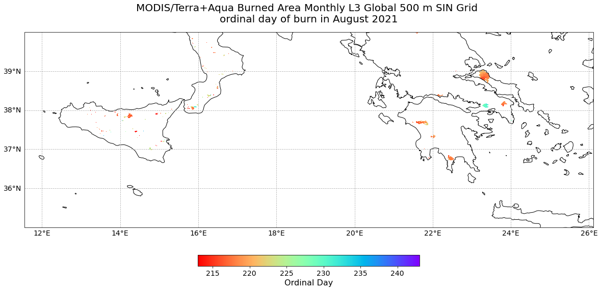
We set the vmin and vmax values to 214 and 244 respectively, which are the ordinal days for the first and last day of the month of August 2021. We set the extent of the plot to highlight burned areas in southern Italy and in Greece.
visualize_pcolormesh(data_array=burndate_data,
                     longitude=lon,
                     latitude=lat,
                     projection=ccrs.PlateCarree(),
                     color_scale='rainbow_r',
                     unit='Ordinal Day',
                     long_name='MODIS/Terra+Aqua Burned Area Monthly L3 Global 500 m SIN Grid \n' + long_name + ' in August 2021',
                     vmin=213,
                     vmax=243,
                     lonmin=lon.min(),
                     lonmax=lon.max(),
                     latmin=35,
                     latmax=lat.max(),
                     set_global=False)
(<Figure size 1440x720 with 2 Axes>,
 <GeoAxesSubplot:title={'center':'MODIS/Terra+Aqua Burned Area Monthly L3 Global 500 m SIN Grid \nordinal day of burn in August 2021'}>)
References
Giglio, L., Justice, C., Boschetti, L., Roy, D. (2021). MODIS/Terra+Aqua Burned Area Monthly L3 Global 500m SIN Grid V061 [Data set]. NASA EOSDIS Land Processes DAAC. https://doi.org/10.5067/MODIS/MCD64A1.061
Some code in this notebook was adapted from the following source:
origin: https://hdfeos.org/zoo/LPDAAC/MCD43A3_A2013305_h12v11_005_2013322102420.py
copyright: 2014, John Evans
license: Public Domain
retrieved: 2022-06-28 by Sabrina Szeto
Return to the case study
Assessing post-fire impacts with next-generation satellites: Mediterranean Fires Case Study
Burn Area Mapping