Metop-B IASI - Total Column Carbon Monoxide - Level 2¶

Hint

Execute the notebook on the training platform >>

The Infrared Atmospheric Sounding Interferometer (IASI) is an instrument onboard the Metop-B/C satellites. It was also previously aboard Metop-A. It provides information on the vertical structure of temperature and humidity as well as main atmospheric species.

This notebook provides you an introduction to data from Metop-B IASI. This dataset is used as a proxy for data from IASI-NG, a passive infrared sounder which has the capability to measure the temperature and water vapour profiles of the Earth’s atmosphere. IASI Level 2 data can be downloaded from the IASI portal.

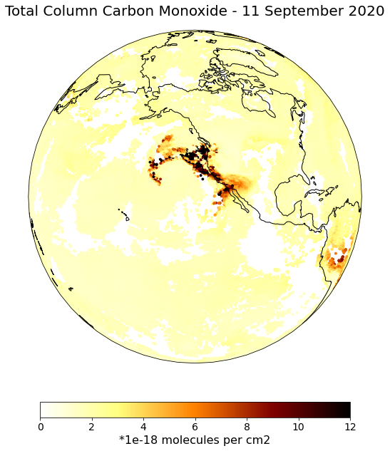
The event featured is the August Complex fire in California, USA in 2020. This was the largest wildfire in CA history, spreading over 1,000,000 acres (over 4,000 sq km).

Basic Facts

Spatial resolution: 4 x 12-km coverage close to the centre of a 48 x 48 km2 cell (average sampling distance: 24 km)
Spatial coverage: Near global
Revisit time: less than one day
Data availability: since 2007

How to access the data

IASI Level 2 are disseminated in the netCDF format and can be downloaded via the IASI portal.

Load required libraries

import os
import xarray as xr
from datetime import datetime
import numpy as np
from netCDF4 import Dataset
import pandas as pd

# Python libraries for visualization
import matplotlib.pyplot as plt
import matplotlib.colors
import matplotlib.cm as cm
from matplotlib.axes import Axes
import cartopy
import cartopy.crs as ccrs
from cartopy.mpl.gridliner import LONGITUDE_FORMATTER, LATITUDE_FORMATTER
from cartopy.mpl.geoaxes import GeoAxes
GeoAxes._pcolormesh_patched = Axes.pcolormesh
from skimage import exposure

import warnings
warnings.filterwarnings('ignore')
warnings.simplefilter(action = "ignore", category = RuntimeWarning)

Load helper functions

%run ../functions.ipynb

Convert units of Total Column Carbon Monoxide data¶

The last step before visualizing the total column carbon monoxide information is to convert the data from mol/m2 to molecules/cm2. The loaded data variable co has an attribute called multiplication_factor_to_convert_to_molecules_per_cm2, which is used to convert the data values.

iasi_co_masked_converted = iasi_co_masked*co.multiplication_factor_to_convert_to_molecules_per_cm2
iasi_co_masked_converted 

<xarray.DataArray (ground_pixel: 392634)>
array([1.7317139e+18, 1.7851012e+18, 1.8219404e+18, ..., 1.9151522e+18,
       2.1212919e+18, 1.8759807e+18], dtype=float32)
Coordinates:
    latitude   (ground_pixel) float32 9.989 10.37 10.54 ... 84.91 84.73 85.22
    longitude  (ground_pixel) float32 -43.75 -41.56 -41.6 ... -66.97 -54.55
Dimensions without coordinates: ground_pixel

Visualize IASI Total Column Carbon Monoxide¶

You can visualize the IASI Total Column Carbon Monoxide data with the function visualize_scatter, which uses matplotlib’s scatterplot function. You can set an Orthographic() projection and focus on a region over California.

visualize_scatter(xr_dataarray=iasi_co_masked_converted, 
                  conversion_factor=1e-18,
                  projection=ccrs.Orthographic(-130,30), 
                  vmin=0, 
                  vmax=12, 
                  point_size=8, 
                  color_scale='afmhot_r', 
                  unit='*1e-18 molecules per cm2', 
                  title='Total Column Carbon Monoxide - 11 September 2020')

../_images/figure3_Metop-B_IASI_L2_CO_34_0.png

References¶

IASI is a joint mission of EUMETSAT and the Centre National d’Etudes Spatiales (CNES, France). The authors acknowledge the AERIS data infrastructure for providing access to the IASI data in this study, ULB-LATMOS for the development of the retrieval algorithms, and Eumetsat/AC SAF for CO data production
Some code in this notebook was adapted from the following source:
- origin: https://gitlab.eumetsat.int/eumetlab/atmosphere/atmosphere/-/blob/master/20_data_exploration/232_Metop-AB_IASI_CO_L2_load_browse.ipynb
- copyright: 2022, EUMETSAT
- license: MIT
- retrieved: 2022-06-28 by Sabrina Szeto

Return to the case study

Monitoring smoke transport with next-generation satellites from Metop-SG: Californian Wildfires Case Study
EPS-SG IASI-NG Carbon Monoxide

FANGS - Fire Applications with Next-Generation Satellites

Metop-B IASI - Total Column Carbon Monoxide - Level 2

Contents

Metop-B IASI - Total Column Carbon Monoxide - Level 2¶

Load and browse IASI Total Column Carbon Monoxide data¶

Retrieve the variable ‘CO total column’ as xarray.DataArray¶

Load data into a xarray.DataArray with the function `generate_xr_from_1d_vec`¶

Mask Total Column Carbon Monoxide data by quality flag¶

Load quality flag information¶

Mask the Total Column Carbon Monoxide data¶

Convert units of Total Column Carbon Monoxide data¶

Visualize IASI Total Column Carbon Monoxide¶

References¶

FANGS - Fire Applications with Next-Generation Satellites

Metop-B IASI - Total Column Carbon Monoxide - Level 2

Contents

Metop-B IASI - Total Column Carbon Monoxide - Level 2¶

Load and browse IASI Total Column Carbon Monoxide data¶

Retrieve the variable ‘CO total column’ as xarray.DataArray¶

Load data into a xarray.DataArray with the function generate_xr_from_1d_vec¶

Mask Total Column Carbon Monoxide data by quality flag¶

Load quality flag information¶

Mask the Total Column Carbon Monoxide data¶

Convert units of Total Column Carbon Monoxide data¶

Visualize IASI Total Column Carbon Monoxide¶

References¶

Load data into a xarray.DataArray with the function `generate_xr_from_1d_vec`¶