Monitoring fires with next-generation satellites from MTG and Metop-SG
Contents
Monitoring fires with next-generation satellites from MTG and Metop-SG
In the near future, new satellites such as Meteosat Third Generation (MTG) and Metop - Second Generation (Metop-SG) will provide advanced capabilities and valuable data for monitoring fires and their impacts. This two-part case study will introduce upcoming data products from MTG and Metop-SG in the context of the 2020 August Complex fire which occurred in California, USA. In this part, we will be focusing on fire monitoring on 11 September 2020 using data products from MTG. In Part 2, we will introduce you to new capabilities in monitoring smoke transport using data products from Metop-SG.
The Case Event
The 2020 August Complex fire was the largest wildfire in California’s history, spreading over 1,000,000 acres (over 4,000 sq km). The fires were caused by a series of lightning strikes on 17 August, resulting in 37 separate fires that merged into a complex. The fires burned for 86 days before being fully contained. On 10 September 2020, CNN reported that the west coast of the US had “the worst air quality in the world” that day, with multiple locations reporting hazardous PM2.5 pollution levels.
Meteosat Third Generation (MTG)
MTG will see the launch of six new geostationary satellites from 2022 onwards. The satellite series will be based on 3-axis platforms and comprise: four imaging satellites (MTG-I) and two sounding satellites (MTG-S). The full operational configuration will consist of two MTG-I satellites operating in tandem, one scanning Europe and Africa every 10 minutes, and the other scanning only Europe every 2.5 minutes, and one MTG-S satellite.
EUMETSAT Polar System - Second Generation (EPS-SG)
The EPS-SG is a partnership programme, which involves the European Space Agency, the German Aerospace Agency and the National Center for Space Studies. The mission is composed of two series of spacecraft, Metop-SG A and B, flying on the same mid-morning orbit, like the current Metop satellites. The orbit height is in the range 823-848 km (dependent on latitudes). There will be three satellites each of Metop-SG A and Metop-SG B. The first two satellites Metop-SG A1 and Metop-SG B1 are planned to be launched in Q2 and Q4 2024 respectively. See here an overview of the planned launch dates.
Consisting of low earth orbiting satellites, Metop-SG will provide high spatial resolution imagery and data. However, they will only cover a smaller observation region and have a longer revisit period compared to geostationary satellites like MTG.
In this case study, we will be focusing on data from several instruments, namely MTG’s Flexible Combined Imager and Metop-SG’s METimage radiometer. We will also be using data from the Sentinel-2 MultiSpectral Instrument to assess burn severity. While data from MTG and Metop-SG is not yet available, we will be using proxy data from existing instruments to demonstrate the new capabilities that will arise from these satellites.
What is proxy data?
Proxy data refers to “data with valid scientific content, to be used in early training on instrument capabilities and application areas, for example in test beds. These are real datasets from relevant existing precursor instruments.” (Source: EUMETSAT)
Monitoring the fire life cycle consists of three stages: (1) pre-fire, (2) active fire and (3) post-fire. First, we can assess pre-fire risk based on meteorological and vegetation conditions. During the fire, we can detect and monitor the location of active fires as well as smoke being produced by the fires. Finally, after the fires have been extinguished, the burned area and burn severity can be assessed.
MTG Flexible Combined Imager
Fire risk mapping
Early information for fire risk is crucial for emergency response. Data from Flexible Combined Imager (FCI) aboard the MTG satellites will be incorporated into fire risk mapping that will enable operational users to plan ahead and allocate resources to mitigate potential fire damage. The FCI provides 16 channels in the visible and infrared spectrum with a spatial sampling distance in the range of 1 to 2 km and four channels with a spatial sampling distance in the range of 0.5 to 1 km.
Figure 1 shows a fire risk map for California on 17 August 2020, when the August Complex Fires were ignited by a lightning storm. The proxy data source is the Wildland Fire Potential Index (WFPI), which integrates meteorological information such as wind speed, dry bulb temperature and rainfall, with satellite-based vegetation condition information to estimate the moisture levels of both live and dead vegetation. The WFPI is a unitless number that ranges from 0 to 150, with higher values indicating higher vegetation flammability. This WFPI is produced by the United States Geological Service (USGS) and is available as a daily forecast for 7 days into the future.
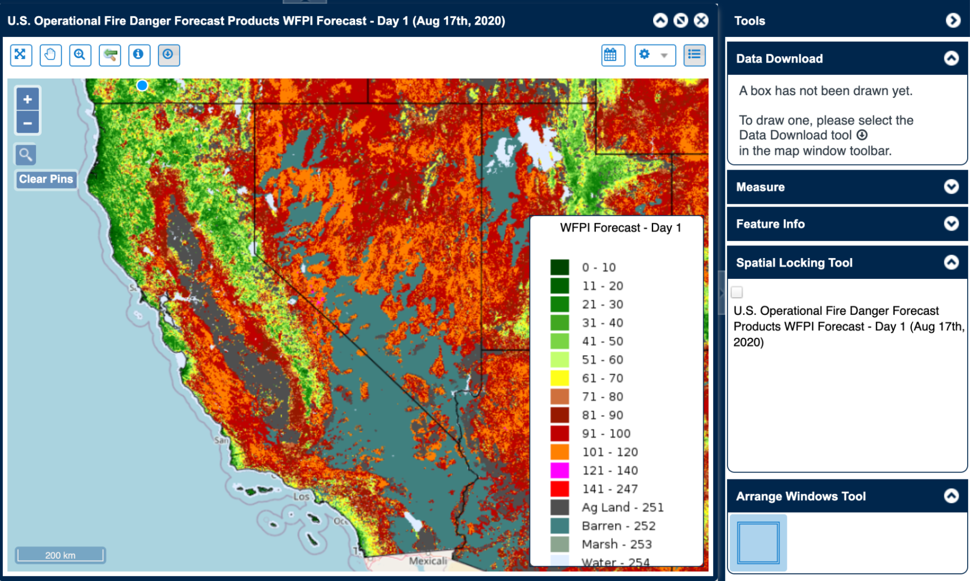
Figure 1. Fire risk map of California on 17th August 2020 from USGS
True colour composite imagery
As the FCI will be capturing data every 10 minutes, it will be possible to have near-real time true colour monitoring of smoke transport and spread of active fires. As an example, Figure 3 shows an animation of the August Complex fires in California recorded on 20 August 2020. The proxy data source is Level 1B surface reflectance data from the GOES-17 ABI instrument.
Figure 2. True colour animation of smoke rising from wildfires along the coast of California on 20 August 2020 recorded by GOES-17 ABI.
Learn how this animation was made.
Fire Radiative Power
In addition, the FCI will also allow for detection and monitoring of characteristics of active fires such as the area that is burning, the temperature of the fires and the rate of the radiative power emitted (also known as the fire radiative power). Fire radiative power is measured in units of power such as watts or megawatts. Figure 3 shows the fire radiative power from the GOES-17 ABI Fire and Hotspot Characterisation product at 22:01 UTC on 20 August 2020. A few high-intensity fires shown in red are producing dense smoke plumes. In the lower-right corner of the image, a cluster of lower intensity fires colored in blue can be seen. This cluster of fires produced a burn scar, shown in Figure 4, which we will investigate further in the next section of this case study.
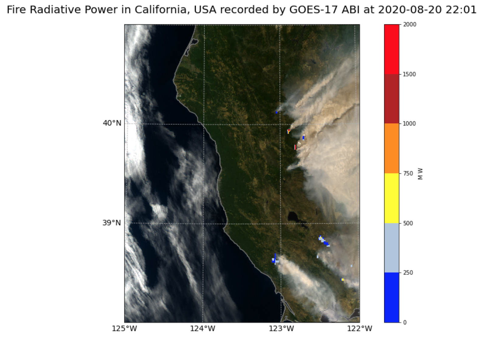
Figure 3. Fire Radiative Power in California, USA overlaid on a true colour composite, recorded by GOES-17 ABI on 20 August 2020.
Learn how this plot of fire radiative power was made.
EPS-SG METimage
Burn Area Mapping
METimage will provide the capability to produce high resolution burn area mapping for post-fire impact assessment. Figure 4 shows burned areas coloured by the ordinal day (the day of the year) that it burned on. The proxy data source is MODIS, which like METimage, has a spatial resolution of 500m. The MODIS Burned Area Monthly Level 3 (MCD64A1) product shows the ordinal day of burn in August 2020. Figure 4 shows a large burn area north of the San Pablo and Suisun bays that resulted from the cluster of lower intensity fires we referred to earlier in Figure 3.
METimage is a multi-spectral (visible and IR) imaging passive radiometer which will provide detailed information on clouds, wind, aerosols and surface properties which are essential for meteorological and climate applications. Compared to its predecessor AVHRR, METimage will have many more channels for the benefit of measuring far more geophysical variables. This combined with on-board radiometric calibration of solar channels and the enhanced spatial sampling (500m compared to 1km at nadir) will provide a breakthrough in several application areas: numerical weather forecast, very short-range forecast and now-casting, oceanography, hydrology, land-surface applications, and climate monitoring.
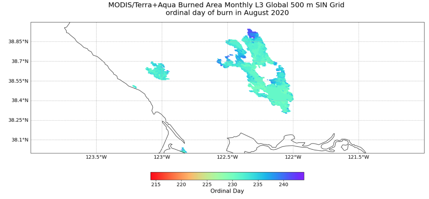
Figure 4. Burned area north of the San Pablo and Suisun bays coloured by the ordinal day of burn in August 2021 from the MODIS Burned Area Monthly Level 3 product.
Learn how this burned area figure showing ordinal day of burn was made.
Sentinel-2
Data from Sentinel-2 is especially useful for assessing burn severity due to its high spatial resolution of up to 10m. This makes it a useful complementary dataset to the data from MTG and Metop-SG. We will now demonstrate several ways that data from Sentinel-2 can be used, including the creation of composite imagery, calculation of a burn index and burn severity mapping.
The Copernicus Sentinel-2 mission comprises a constellation of two polar-orbiting satellites placed in the same sun-synchronous orbit, phased at 180° to each other. It aims at monitoring variability in land surface conditions, and its wide swath width (290 km) and high revisit time (10 days at the equator with one satellite, and 5 days with 2 satellites under cloud-free conditions which results in 2-3 days at mid-latitudes) will support monitoring of Earth’s surface changes.
Sentinel-2 MultiSpectral Instrument
The Sentinel-2 MultiSpectral Instrument (MSI) has 13 spectral bands which provide data for land cover/change classification, atmospheric correction and cloud/snow separation. The MSI samples four bands at 10 m, six bands at 20 m and three bands at 60 m spatial resolution. Due to the high spatial resolution of up to 10m, the Sentinel-2 MSI data is useful for creating image composites. MSI data products include top-of-atmosphere reflectances (Level 1C data) and bottom-of-atmosphere reflectances (Level 2A data).
Natural colour composites
Natural colour composites are similar to what the human eye would see. To create a natural colour composite, one can assign the red, green and blue channels of image to show the corresponding visible red, visible green and visible blue bands of the satellite data. Figure 5 shows natural colour composites from Sentinel-2 Level 2A data on two dates. The left image was taken before the fires on 7 August 2020 and the image on the right was taken after the fires were extinguished on 25 November 2020. The water bodies visible near the bottom of the images are the San Pablo and Suisun Bays.
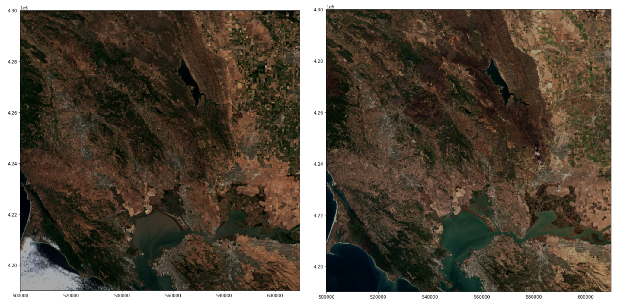
Figure 5. Natural colour composites from Sentinel-2 Level 2A data showing pre-fire conditions on 7 August 2020 (left) and post-fire conditions on 25 November 2020 (right) in California, USA.
Learn how these Natural colour composites were made.
False colour composites
The burn scars from the fires are not easily seen in the natural colour images in Figure 5. However, we can also create a false colour composite that makes burn scars more easily distinguishable. The recipe for the false colour composites is: Red-Green-Blue 12-8A-2. This means that the red channel was assigned to band 12 (shortwave infrared), the green channel was assigned to band 8A (near-infrared) and the blue channel was assigned to band 2 (the visible blue band). This recipe highlights burn scars in brown and healthy vegetation in green.
Figure 6 shows two false colour composites created from the Sentinel-2 MSI data captured on the same dates as before. The left image was taken before the fires on 7 August 2020 and the image on the right was taken after the fires were extinguished on 25 November 2020. In the false colour composite from November 2020, a large brown burn scar around Lake Berryessa is clearly visible. This is the same burn scar you can see in Figure 4.
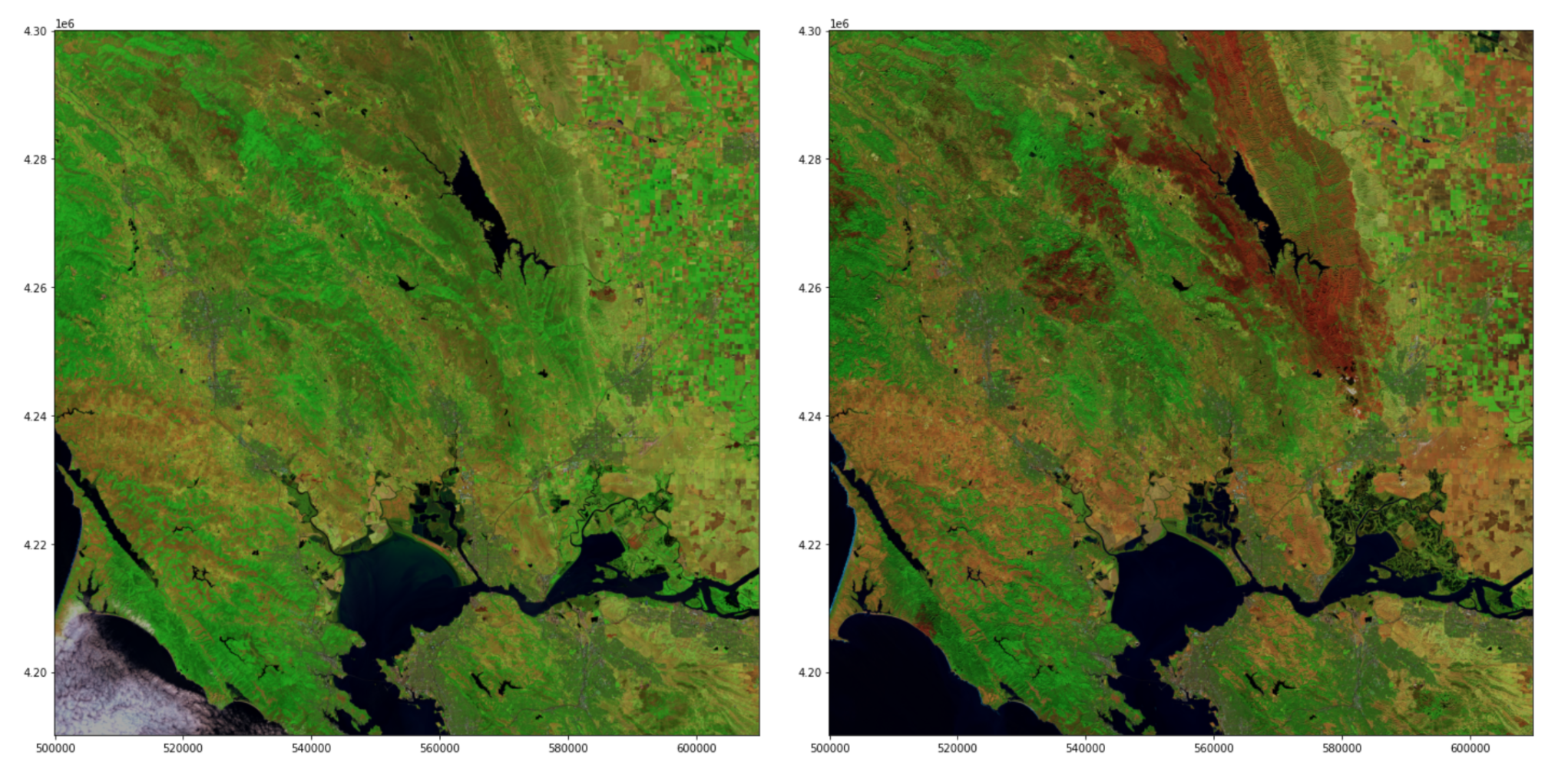
Figure 6. False colour composites from Sentinel-2 Level 2A data showing pre-fire conditions on 7 August 2020 (left) and post-fire conditions on 25 November 2020 (right) in California, USA.
Learn how these False colour composites were made.
Normalised Burn Ratio (NBR)
In order to assess burn severity, we can calculate the Normalised Burn Ratio (NBR). As explained by UN SPIDER, the NBR “uses near-infrared (NIR) and shortwave-infrared (SWIR) wavelengths. Healthy vegetation before the fire has very high NIR reflectance and a low SWIR response. In contrast, recently burned areas have a low reflectance in the NIR and high reflectance in the SWIR band.” The formula is NBR = (NIR - SWIR) / (NIR + SWIR) or using the MSI band numbers: NBR = (B8A - B12) / (B8A + B12).
Next, “The NBR is calculated for images before the fire (pre-fire NBR) and for images after the fire (post-fire NBR) and the post-fire image is subtracted from the pre-fire image to create the differenced (or delta) NBR (dNBR) image. dNBR can be used for burn severity assessment, as areas with higher dNBR values indicate more severe damage whereas areas with negative dNBR values might show increased vegetation productivity. dNBR can be classified according to burn severity ranges proposed by the United States Geological Survey (USGS).”
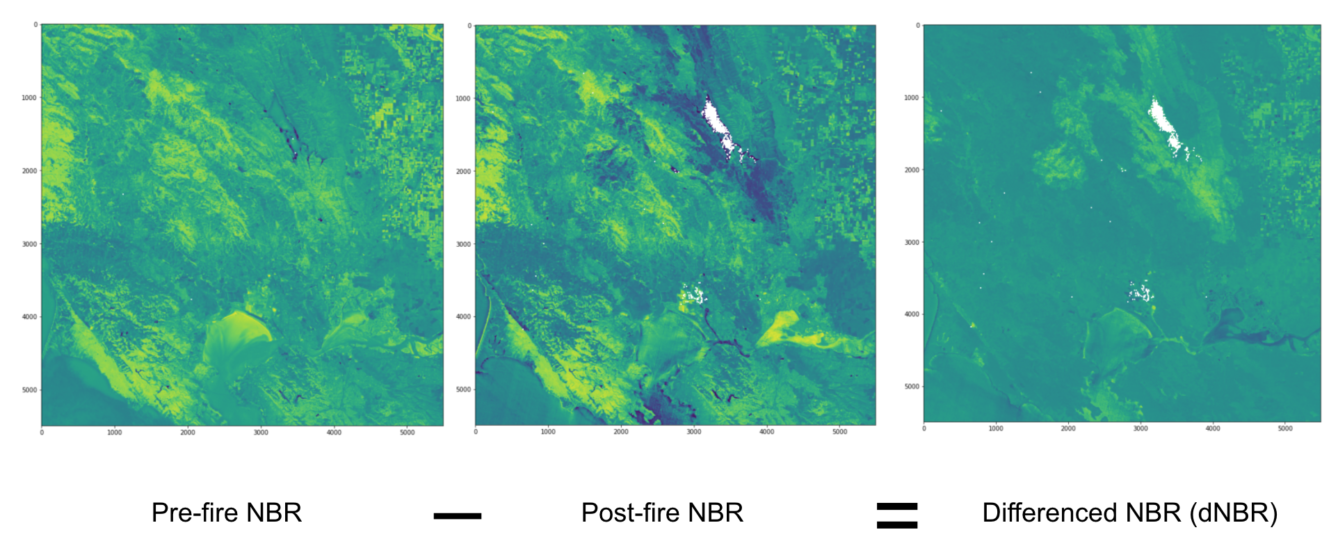
Figure 7. The Differenced Normalised Burn Ratio (dNBR) image (right) is calculated from Sentinel-2 Level 2A data by subtracting the pre-fire NBR on 7 August 2020 (left) from the post-fire NBR on 25 November 2020 (middle).
Learn how the Normalized Burn Ratio (NBR) and Differenced NBR images were made.
Burn Severity Map
As shown in Figure 8, dNBR can be classified according to burn severity ranges proposed by the USGS. The water bodies are also masked using the water mask from the Sentinel-2 data’s scene classification layer. The burn scar around Lake Berryessa has been classified as having areas with both high and moderate-high severity burns. Note that the rectangular-shaped fields on the right side of the image are likely to have been harvested, leading to a false classification as having a high severity burn.
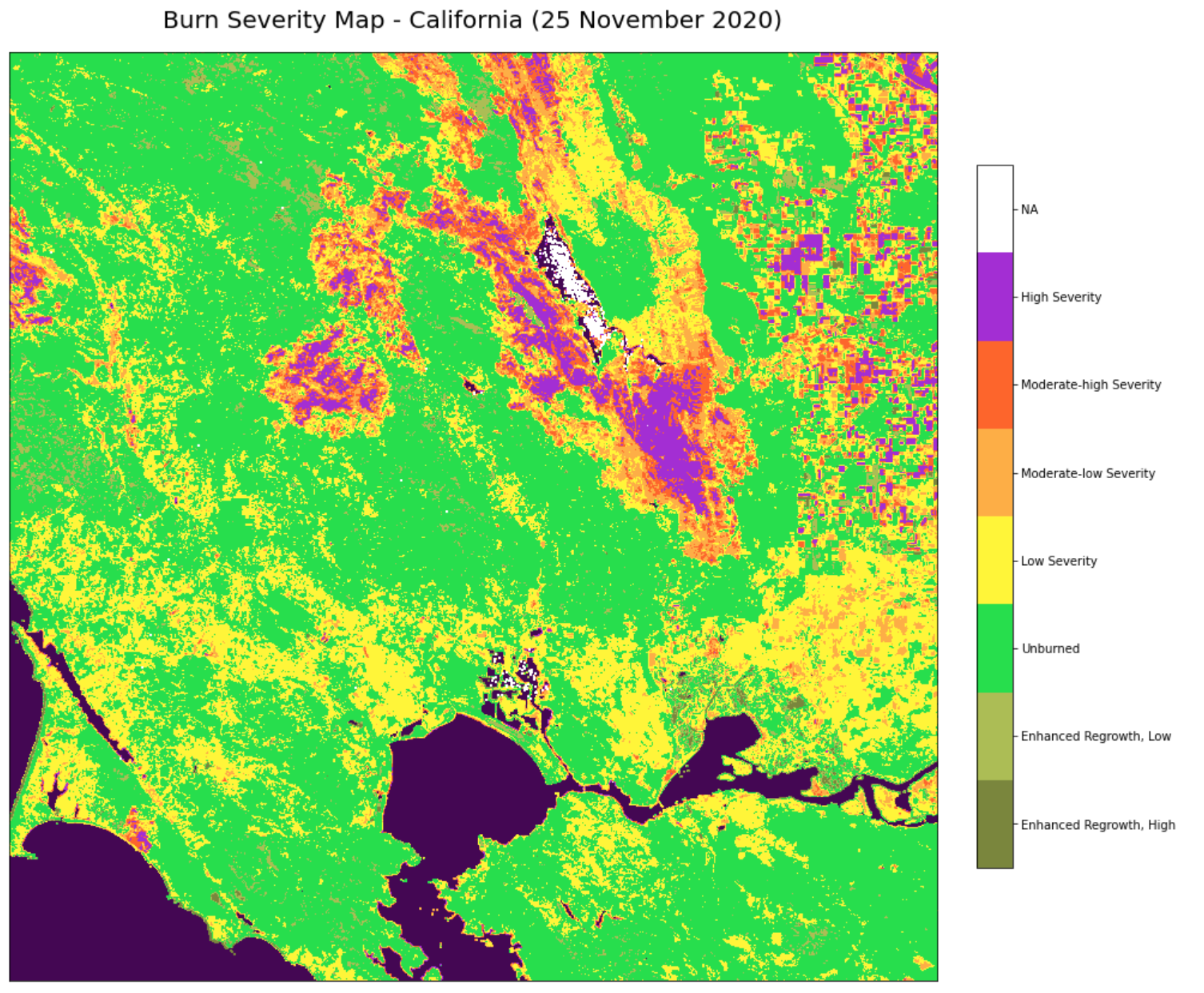
Figure 8. Burn severity is classified using the dNBR image shown in Figure 7. The coastal water bodies are masked using the water mask from the Sentinel-2 data’s scene classification layer.
Learn how this Burn severity map was made.
References
USGS Wildland Fire Potential Index, https://www.usgs.gov/fire-danger-forecast/wildland-fire-potential-index-wfpi
GOES-R Calibration Working Group and GOES-R Series Program. (2017). NOAA GOES-R Series Advanced Baseline Imager (ABI) Level 1b Radiances. NOAA National Centers for Environmental Information. doi:10.7289/V5BV7DSR.
GOES-R Calibration Working Group and GOES-R Series Program. (2017). NOAA GOES-R Series Advanced Baseline Imager (ABI) Level 2 fire and Hotspot Characterisation. NOAA National Centers for Environmental Information. doi:10.7289/V5BV7DSR.
Giglio, L., Justice, C., Boschetti, L., Roy, D. (2015). MCD64A1 MODIS/Terra+Aqua Burned Area Monthly L3 Global 500m SIN Grid V006 [Data set]. NASA EOSDIS Land Processes DAAC. https://doi.org/10.5067/MODIS/MCD64A1.006
Copernicus Sentinel data 2020